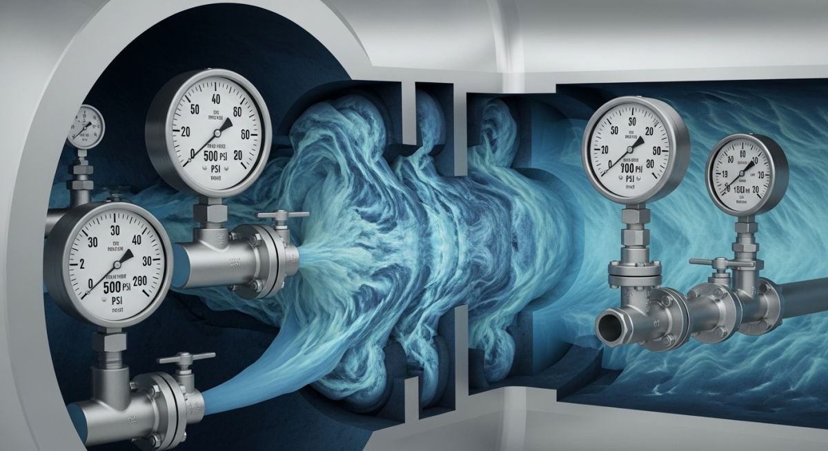
Hydraulic Calculation in Piping Networks: A Technical Guide
In my two decades of experience, I have seen countless projects stall during the commissioning phase simply because the initial hydraulic analysis failed to account for minor losses or fluid property variations. Accurate hydraulic calculation in piping networks is not merely a design exercise; it is the foundation of operational safety and pump efficiency.
Whether you are sizing a new refinery header or troubleshooting a legacy cooling water loop, understanding the interplay between friction factors, Reynolds numbers, and pipe roughness is non-negotiable. This guide breaks down the rigorous methodologies required to model these systems effectively.
Key Takeaways for Piping Engineers:
- Mastering the Darcy-Weisbach equation for high-accuracy pressure drop modeling.
- Applying the Hazen-Williams method for water-based utility systems.
- Optimizing flow velocities to prevent erosion and excessive noise.
- Integrating ASME B31.3 requirements into your hydraulic design basis.
Advanced Hydraulic Calculation in Piping Networks
Hydraulic Analysis Methodology: The rigorous application of fluid mechanics principles to predict pressure gradients and flow distribution across complex piping topologies.
When performing a hydraulic calculation in piping networks, the primary objective is to balance the energy equation between two points. We utilize the Darcy-Weisbach equation as our primary tool for all fluid types, as it provides a more robust physical basis than empirical alternatives. The pressure drop is defined by the friction factor, pipe length, diameter, and the square of the fluid velocity.
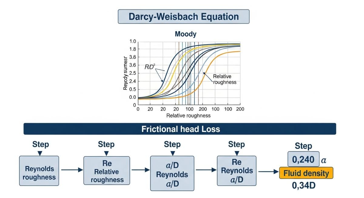
The Darcy-Weisbach Framework
The head loss due to friction is calculated using the formula where head loss equals the friction factor multiplied by the ratio of pipe length to diameter, multiplied by the velocity head. For laminar flow, the friction factor is simply 64 divided by the Reynolds number. However, in most industrial piping, we operate in the turbulent regime, requiring the Colebrook-White equation to solve for the friction factor iteratively.
Field Warning: Minor Loss Neglect
A common error I encounter is the omission of minor losses from valves, fittings, and instrumentation. In complex networks, these can account for up to 30 percent of the total pressure drop. Always apply the K-factor method or the equivalent length method to ensure your pump head requirements are not underestimated.
Velocity Limits and ASME Compliance
Velocity management is critical to prevent erosion-corrosion, particularly in carbon steel piping carrying corrosive fluids. I typically adhere to the API RP 14E guidelines for velocity limits, which suggest that the erosional velocity is a function of the fluid density and the empirical constant C. Exceeding these limits leads to premature wall thinning, which directly violates the safety margins mandated by ASME B31.3.
Furthermore, when dealing with compressible fluids like natural gas or steam, the hydraulic calculation must account for density changes along the pipe length. Using an isothermal or adiabatic flow model is necessary when the pressure drop exceeds 10 percent of the inlet pressure. Failure to account for these compressibility effects will result in inaccurate flow rate predictions and potential system instability.
Hydraulic Modeling Trade-offs: A comparative analysis of analytical methods and their practical limitations in industrial piping design.
Advantages
- Darcy-Weisbach provides high accuracy across all fluid regimes.
- Enables precise pump sizing, reducing energy consumption and operational costs.
- Facilitates early identification of potential cavitation risks in control valves.
- Ensures compliance with ASME B31.3 pressure containment requirements.
- Allows for sensitivity analysis of fluid property variations during process upsets.
Disadvantages
- Iterative calculations for friction factors require specialized software for large networks.
- Hazen-Williams is often misused for non-water fluids, leading to significant errors.
- High sensitivity to pipe roughness assumptions in aging infrastructure.
- Complexity increases exponentially with the number of parallel branches and loops.
- Requires accurate, up-to-date P&IDs to avoid modeling incorrect fitting counts.
Industrial Hydraulic Implementation: Practical scenarios where precise hydraulic calculation in piping networks dictates system performance and safety.
High-Pressure Steam Distribution
In steam networks, hydraulic calculations must account for phase changes and high-velocity flow. We utilize these models to size condensate removal systems and prevent water hammer, ensuring the piping remains within the stress limits defined by ASME B31.1.
Cooling Water Loop Optimization
Large-scale cooling loops require balancing flow across multiple heat exchangers to maintain thermal efficiency. By calculating the pressure drop across each branch, we can install orifice plates or control valves to ensure the design flow rate is achieved at every terminal point.
Hydrocarbon Pipeline Transport
For long-distance liquid transport, hydraulic analysis determines the spacing of booster pump stations. We model the viscosity-temperature relationship to predict the pressure gradient, which is vital for maintaining the integrity of the pipeline under varying seasonal ambient conditions.
When performing a rigorous hydraulic calculation in piping networks, the selection of the friction factor is the most significant variable influencing the accuracy of your pressure drop prediction. For turbulent flow regimes, the Colebrook-White equation remains the gold standard, though it requires iterative numerical methods due to its implicit nature. In my two decades of field experience, I have observed that engineers often default to simplified charts, which can lead to significant underestimation of head loss in aging systems where internal pipe roughness has increased due to corrosion or scaling.
The following table provides a comparative overview of friction factor estimation methods and their applicability based on the Reynolds number and relative roughness. It is imperative to note that for ASME B31.3 compliant systems, the choice of method must be documented in the design basis. Always verify the absolute roughness values against the specific material specifications provided by the pipe manufacturer, as variations in manufacturing processes can alter the effective friction coefficient significantly.
| Methodology | Reynolds Range | Complexity | Primary Application |
|---|---|---|---|
| Blasius Equation | Less than 100,000 | Low | Smooth pipes |
| Colebrook-White | All Turbulent | High | General Process Piping |
| Haaland Equation | All Turbulent | Medium | Explicit Approximation |
By utilizing these methods, you ensure that the hydraulic calculation in piping networks accounts for the non-linear relationship between velocity and energy dissipation. Always cross-reference your calculated pressure drop with the pump performance curves to avoid cavitation risks.
Effective hydraulic analysis requires a structured approach to data management. In my practice, I maintain a matrix that links physical fluid properties with the governing mechanical standards. This ensures that every hydraulic calculation in piping networks is traceable to a specific code requirement, such as ASME B31.3 for process piping or API 5L for line pipe specifications.
The matrix below categorizes the critical entities involved in fluid transport modeling. By mapping these parameters, you can quickly identify which variables are sensitive to temperature fluctuations or pressure surges. This systematic approach prevents the common pitfall of using static fluid properties for dynamic system analysis, which often leads to undersized piping or excessive pump power consumption.
| Entity | Standard | Parameter |
|---|---|---|
| Fluid Density | ISO 1183 | Mass per unit volume |
| Pipe Roughness | ASME B31.3 | Internal surface profile |
| Viscosity | ASTM D445 | Dynamic/Kinematic resistance |
This matrix serves as a foundational tool for any hydraulic calculation in piping networks, ensuring that your design remains robust across varying operational conditions and fluid compositions.
Performing a hydraulic calculation in piping networks is only half the battle; the real-world installation must match the design intent. I have seen countless projects fail because the as-built piping configuration deviated from the isometric drawings used in the initial hydraulic model. This checklist is designed to bridge the gap between theoretical calculations and physical site reality.
-
1.
Verify that all valves are fully open and that the valve type (gate vs. globe) matches the hydraulic model assumptions. -
2.
Confirm that the internal pipe diameter matches the nominal bore used in the pressure drop calculation, accounting for schedule thickness. -
3.
Inspect for any unauthorized field-routed bends or elbows that were not included in the original equivalent length calculations. -
4.
Check for debris or construction residue that could increase the effective roughness coefficient beyond the design value. -
5.
Validate that the pump suction and discharge pressure gauges are calibrated and located at the exact points modeled in the software.
When conducting these checks, prioritize the high-velocity sections of the network. Any discrepancy in these areas will have a disproportionate impact on the overall system performance. If you find that the measured pressure drop significantly exceeds your calculated values, revisit the ASME B31.3 guidelines regarding flow velocity limits to ensure that the system is not operating in a regime that promotes erosion or excessive turbulence. Always document these findings in your final commissioning report to maintain a clear audit trail for future maintenance and system upgrades.
Field Case Study: Real-World Application
The Problem: Unexpected Pressure Drop in a Cooling Water Loop
A major petrochemical facility reported a 15% reduction in flow rate despite the pump operating at its rated speed. The initial hydraulic calculation in piping networks had predicted a much lower pressure drop, leading to concerns about pump degradation.
- Accumulation of bio-fouling on the internal pipe walls.
- Incorrect assumption of pipe roughness in the original design.
- Presence of partially closed isolation valves in the bypass line.
- Increased fluid viscosity due to heat exchanger efficiency loss.
The Outcome: Restoring System Performance
By re-evaluating the hydraulic model with updated roughness values and performing a physical inspection, we identified the root cause and restored the system to its design capacity.
- Achieved a 12% increase in flow rate after chemical cleaning.
- Validated the updated hydraulic model against real-time sensor data.
- Implemented a new maintenance schedule for internal pipe inspection.
- Reduced pump energy consumption by optimizing the operating point.
My recommendation for similar scenarios is to always perform a sensitivity analysis on your roughness parameters. A small change in the internal surface condition can lead to a significant shift in the system curve, especially in long-distance piping networks where friction losses dominate the total head requirement.
Frequently Asked Engineering Questions
How does pipe roughness affect hydraulic calculation in piping networks?
- Higher roughness values directly increase the friction factor.
- Increased friction leads to a steeper system curve.
- Calculations must account for aging to ensure long-term pump viability.
What is the role of the Reynolds number in hydraulic analysis?
- Laminar flow occurs at low Reynolds numbers, where viscous forces dominate.
- Turbulent flow occurs at high Reynolds numbers, where inertial forces dominate.
- The friction factor calculation method changes significantly based on this regime.
Why is ASME B31.3 important for hydraulic design?
- Ensures structural integrity under pressure and temperature.
- Standardizes the approach to pressure drop and velocity limits.
- Provides a legal framework for safe industrial operation.
How do I calculate pressure drop in complex piping networks?
- Sum the pressure drops across all parallel and series paths.
- Ensure mass balance at every junction point.
- Account for minor losses from fittings and valves using equivalent length factors.
What are the velocity limits for process piping?
- Liquid service: Typically 1 to 3 meters per second to avoid erosion.
- Gas service: Often limited to 20 to 50 meters per second to prevent noise.
- Always check project-specific specifications for material-dependent limits.
Can I use Hazen-Williams for all fluids?
- Limited to water-like fluids.
- Inaccurate for high-viscosity hydrocarbons or non-Newtonian fluids.
- Use Darcy-Weisbach for general process applications to ensure accuracy.
📚 Recommended Resources: Hydraulic Calculation in Piping Networks
Read these Guides
🎥 Watch Tutorials

Complete Course on
Piping Engineering
Check Now
Key Features
- 125+ Hours Content
- 500+ Recorded Lectures
- 20+ Years Exp.
- Lifetime Access
Coverage
- Codes & Standards
- Layouts & Design
- Material Eng.
- Stress Analysis