Table of Contents
What is the Reynolds Number? The Equation and Significance
In my 20-plus years of commissioning industrial piping networks and troubleshooting hydraulic bottlenecks, I have seen many young engineers overlook a fundamental truth: fluids do not always behave the way your steady-state software predicts. I remember a project in a heavy crude processing facility where a pump was constantly vibrating, and the piping was rattling like a freight train. The design team had sized the lines based on simple velocity limits, completely ignoring how temperature drops spiked the fluid’s viscosity. When we finally calculated the actual flow dynamics, we discovered the system was operating right in the unstable transition zone.
Understanding this dimensionless value is not just an academic exercise; it is a field survival skill. It dictates your pressure drop, your pump selection, your heat transfer coefficients, and even the rate of localized corrosion in your elbows. Let us break down the mechanics of this critical parameter so you can design systems that run quietly, efficiently, and safely.
- The parameter acts as a direct ratio of momentum-driven inertial forces to friction-driven viscous forces.
- Flow regimes in circular pipes are strictly classified into laminar, transitional, and turbulent zones based on specific numerical thresholds.
- Accurate calculations prevent catastrophic piping fatigue, localized erosion-corrosion, and pump cavitation.
Complete Course on
Piping Engineering
Check Now
Key Features
- 125+ Hours Content
- 500+ Recorded Lectures
- 20+ Years Exp.
- Lifetime Access
Coverage
- Codes & Standards
- Layouts & Design
- Material Eng.
- Stress Analysis
What is the Reynolds Number in Fluid Systems?
Reynolds Number Definition: The dimensionless ratio of inertial forces to viscous forces determines whether fluid flow behaves in a highly ordered laminar fashion or a chaotic turbulent state.
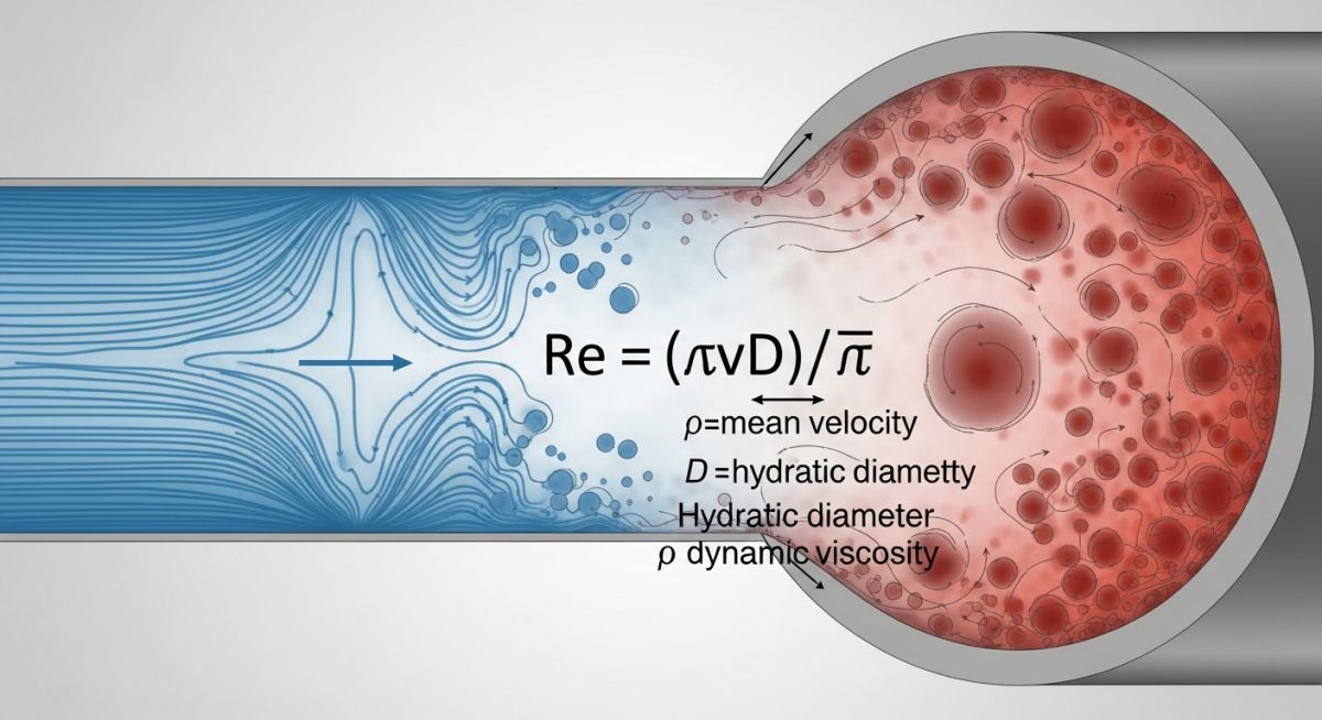
When fluid flows through a pipe, two opposing forces battle for dominance. On one side, you have inertial forces, which represent the fluid’s momentum—its desire to keep moving in a straight line at high velocity. On the other side, you have viscous forces, which act as internal friction, trying to shear the fluid layers and keep them sliding smoothly past one another.
When viscous forces dominate, the fluid flows in neat, parallel layers without lateral mixing. This is laminar flow. When inertial forces take over, the fluid particles move in chaotic, intersecting paths, creating eddies and vortices. This is turbulent flow. The transition between these states is governed by this single dimensionless value, first popularized by Osborne Reynolds in 1883.
The Equation for Reynolds Number Calculations
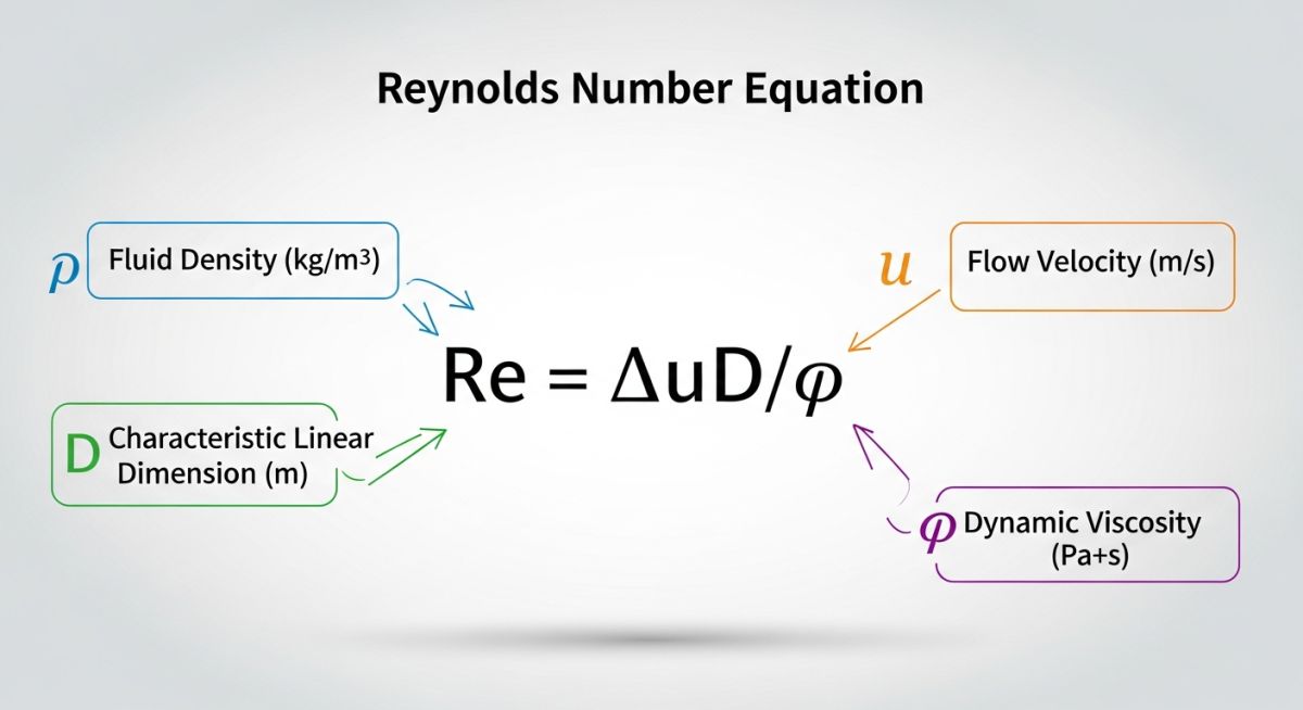
Reynolds Number Equation: The mathematical expression relates fluid density, velocity, characteristic pipe diameter, and dynamic viscosity to establish flow characteristics.
To calculate this value for a fluid flowing through a fully running circular pipe, we use the following standard formula:
Alternatively, if you are working with kinematic viscosity, the formula simplifies to:
Where the variables are defined as:
- ρ (Rho): Fluid density (kg/m³ or lb/ft³)
- u: Mean fluid velocity (m/s or ft/s)
- D: Inside diameter of the pipe (m or ft)
- μ (Mu): Dynamic (absolute) viscosity (Pa·s, kg/(m·s), or lb/(ft·s))
- ν (Nu): Kinematic viscosity (m²/s or ft²/s), where ν = μ / ρ
Factors Affecting Reynolds Number Values
Flow Regime Drivers: Variations in fluid temperature, pipe roughness, and velocity profiles directly alter the viscous and inertial balance within the system.
In my field experience, temperature is the most volatile variable. For liquids, an increase in temperature decreases viscosity, which spikes your calculation and can push a stable laminar flow into a turbulent regime. For gases, the opposite occurs; heating a gas increases its dynamic viscosity, which actually lowers the calculated value.
Never assume viscosity remains constant across your piping run. In outdoor installations, solar radiation or winter ambient drops can alter fluid temperatures enough to shift your flow regime entirely, leading to unexpected pressure drops or control valve hunting.
Reynolds Number Values and Flow Regimes
Flow Regime Boundaries: Specific numerical thresholds define the transition from laminar to turbulent flow in closed conduits.
In piping design, we categorize flow into three distinct zones. These boundaries are critical when applying friction factor equations like the Colebrook-White or Haaland equations for pressure drop calculations.
| Flow Regime | Numerical Range | Flow Characteristics | Design Implications |
|---|---|---|---|
| Laminar Flow | Re < 2,000 | Smooth, parallel streamlines; minimal mixing; viscous forces dominate. | Predictable pressure drop; friction factor f = 64/Re; ideal for high-viscosity polymers. |
| Transitional Flow | 2,000 ≤ Re ≤ 4,000 | Unstable; fluctuates between laminar and turbulent behavior. | Avoid in design; highly unpredictable pressure drops and flow control instability. |
| Turbulent Flow | Re > 4,000 | Chaotic eddies; rapid mixing; inertial forces dominate. | High heat transfer; high pressure drop; requires Moody chart or Colebrook equation. |
To assist in system design, this matrix maps fluid properties, dimensionless relationships, and relevant industry standards.
| Fluid Type | Typical Re Range | Primary Standard | Key Dimensionless Link |
|---|---|---|---|
| Water (Utility Lines) | 10,000 to 500,000 | ASME B31.3 | Directly impacts Nusselt Number (Nu) for heat exchangers. |
| Heavy Crude Oil | 100 to 1,800 | API RP 14E | Determines pump power requirements in laminar regimes. |
| Superheated Steam | 500,000+ | ASME B31.1 | Linked to Mach Number for high-velocity compressibility checks. |
Verifying Reynolds Number in Field Designs
Field Verification Protocol: On-site validation of fluid properties and flow rates ensures that hydraulic calculations match actual operating conditions.
Before finalizing any pump selection or piping layout, I run through this checklist on-site to ensure our theoretical calculations align with physical reality.
-
Verify Operating Temperature: Measure fluid temperature at the inlet and outlet to adjust dynamic viscosity values. -
Confirm Actual Pipe ID: Cross-reference nominal pipe size with schedule thickness (e.g., Schedule 40 vs. Schedule 80) to get the exact internal diameter. -
Check for Non-Newtonian Behavior: Ensure the fluid does not exhibit shear-thinning or shear-thickening properties that invalidate standard formulas. -
Inspect Upstream Disturbances: Ensure there are at least 10 diameters of straight pipe upstream of flow meters to allow the velocity profile to stabilize. -
Validate Flow Meter Calibration: Confirm the flow meter is calibrated for the specific density and viscosity of the process fluid.
Field Case Study: Real-World Application
A heavy crude oil pipeline was experiencing massive, unexplained pressure drops and severe pump cavitation during winter operations. The original design team had assumed a constant laminar flow regime (Re ≈ 1,200) based on summer fluid properties. However, when winter temperatures dropped the oil temperature from 40°C to 12°C, the dynamic viscosity increased by over 300%. This shifted the flow into an extremely viscous laminar state, requiring three times the design pumping power, while localized high-velocity bypass loops went turbulent (Re ≈ 5,500), causing rapid erosion-corrosion at the elbows.
I led the team in recalculating the system hydraulics across the full seasonal temperature envelope. We installed targeted heat tracing to maintain the oil temperature above 25°C, keeping the viscosity within a manageable range. Additionally, we resized the bypass loops to ensure the calculated value never exceeded 1,500. This modification stabilized the flow, eliminated the pump cavitation, and reduced overall energy consumption by 38%.
This case highlights why we must never design for a single point on a graph. Fluid systems are dynamic, and this dimensionless parameter is your primary tool for mapping those dynamics across real-world operating envelopes.
Frequently Asked Engineering Questions
What is the physical significance of a high Reynolds number?
Why is the Reynolds number dimensionless?
How does pipe roughness affect the critical transition point?
What is the difference between dynamic and kinematic viscosity in the formula?
How does this parameter relate to the Darcy friction factor?
Can this calculation be applied to non-Newtonian fluids?

📚 Recommended Resources: Reynolds Number
Related posts:
![A mechanical sucker rod pumpjack operating in an oil field at sunset]()
What is Sucker Rod Pump System in Oil Production?
![Piping material engineer reviewing technical specifications on a tablet in an industrial plant.]()
How a Piping Material Engineer Drives Industrial Project Success
![Industrial refinery plant showing various types of static equipment]()
What is Static Equipment? Types and List of Static Equipments
![Side-by-side comparison of industrial process piping and power plant steam piping systems.]()
Differences Between ASME B31.3 and B31.1: B31.3 vs B31.1
![Large industrial steel storage tank under construction with cranes and scaffolding]()
Storage Tank Construction Method Statement: Step-by-Step Engineering Guide
![Cutaway diagram of a globe control valve highlighting the internal valve trim components]()
What is a Valve Trim? Types, Components, and Selection