Table of Contents
Hooke’s Law: Statement, Equation, Graph, Applications, Limitations
In my 20 years of piping stress analysis, I have seen many young engineers treat Hooke’s Law as a simple high school physics equation. However, when you are designing a high-pressure steam line at 500°C supported by variable spring hangers, this law is the thin line between a safe plant and a catastrophic piping rupture. Understanding how materials deform elastically under load is the bedrock of structural integrity.
Whether we are calculating the cold-to-hot travel of a spring support or verifying the thermal expansion stresses in an ASME B31.3 piping system, we rely on the linear relationship between force and displacement. In this comprehensive guide, I will break down the mathematics, the stress-strain graph, the practical applications, and the physical boundaries of this foundational engineering principle.
Key Engineering Takeaways
- Linear Elasticity: Hooke’s Law only applies within the proportional limit of a material, beyond which plastic deformation occurs.
- Dual Formulations: The law is expressed as F = -kx for discrete spring elements and σ = Eε for continuous solid materials.
- Piping Design Utility: It forms the mathematical basis for sizing variable spring hangers and calculating thermal expansion stresses.
Complete Course on
Piping Engineering
Check Now
Key Features
- 125+ Hours Content
- 500+ Recorded Lectures
- 20+ Years Exp.
- Lifetime Access
Coverage
- Codes & Standards
- Layouts & Design
- Material Eng.
- Stress Analysis
What is Hooke’s Law?
Hooke’s Law Definition: This mechanical principle establishes that the deformation of an elastic body is linearly proportional to the force causing it. It serves as the foundational framework for analyzing structural elasticity, piping thermal expansion, and spring hanger design across industrial engineering applications.
Discovered by the 17th-century British physicist Robert Hooke in 1676, the law was originally published as a Latin anagram, “ut tensio, sic vis“, which translates to “as the extension, so the force”. In practical terms, if you double the load on an elastic object, its displacement or deformation will also double. This predictable behavior is what allows us to design reliable mechanical systems that can withstand cyclic operational loads without suffering permanent structural damage.
Hooke’s Law Statement for Springs
Spring Elasticity Principle: This physical law dictates that the force required to compress or extend a spring is directly proportional to the distance of displacement. It governs the design of variable and constant spring hangers used to support piping systems undergoing thermal movement.
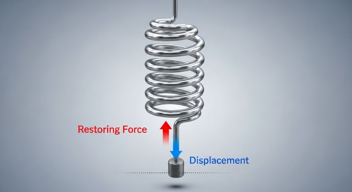
When applied to a discrete mechanical spring, the law states that the magnitude of the force exerted by the spring is directly proportional to its displacement from its free, unstressed length. This relationship is highly linear for standard helical coil springs, making them excellent components for load support and force measurement.
Hooke’s Law Equation for Spring
Spring Force Equation: This mathematical expression calculates the restoring force exerted by a spring when it is displaced from its equilibrium position. It defines the linear relationship between force, displacement, and the spring constant.
To calculate the force associated with spring deformation, we use a straightforward linear equation that links the physical properties of the spring to the distance it is stretched or compressed.
Understanding the Spring Equation F = -kx
Restoring Force Formula: This equation represents the restoring force where the negative sign indicates that the force acts in the opposite direction of the displacement. It ensures that the spring always pulls or pushes back toward its neutral state.
The mathematical formula is written as:
Where:
- F is the restoring force exerted by the spring (measured in Newtons, N).
- k is the spring constant or stiffness (measured in N/mm or N/m), which represents the rigidity of the spring.
- x is the displacement vector representing the distance and direction the spring is deformed from its equilibrium position (measured in mm or m).
In structural and piping design software like CAESAR II, we often omit the negative sign when calculating the external support loads acting on the piping nozzles, focusing instead on the absolute force magnitude transferred to the structural steel.
Hooke’s Law Statement relating Stress & Strain
Stress-Strain Elastic Relationship: This formulation of Hooke’s Law states that stress is directly proportional to strain within the elastic limit of a material. It allows engineers to predict structural deformation and material integrity under mechanical loads.
While the spring equation works perfectly for discrete components, continuous solid materials like steel pipes, pressure vessels, and structural beams require a localized formulation. In solid mechanics, Hooke’s Law is restated to relate internal intensity of force (stress) to the relative deformation (strain) at any given point within the material.
Hooke’s Law Formula for Materials
Elastic Modulus Formula: This equation defines the linear relationship between stress and strain using Young’s Modulus as the constant of proportionality. It is the primary equation used in finite element analysis and piping stress calculations.
This localized version of the law removes geometric dependencies (like length and cross-sectional area), allowing us to evaluate material behavior independently of the component’s physical shape.
Understanding the Stress Equation σ = Eε
Stress Strain Equation: This mathematical representation calculates the internal stress of a material based on its elastic modulus and strain. It forms the basis for determining structural safety margins under ASME B31.3 piping codes.
The material-specific formula is expressed as:
Where:
- σ (Sigma) is the normal stress (measured in MPa or N/mm²).
- E is Young’s Modulus or the Modulus of Elasticity (measured in GPa or MPa), representing material stiffness.
- ε (Epsilon) is the dimensionless strain, calculated as the change in length divided by the original length (ΔL / L).
In high-temperature piping design, Young’s Modulus (E) is not a constant. For instance, ASTM A106 Grade B carbon steel has an elastic modulus of approximately 203 GPa at 20°C, but this drops to about 170 GPa at 400°C. Failing to derate Young’s Modulus in your stress analysis software will lead to underestimating thermal expansion forces, potentially causing piping support failures or over-stressed equipment nozzles. Always reference ASME B31.3 Section II, Part D for temperature-dependent material properties.
Analyzing the Hooke’s Law Graph
Stress-Strain Curve Analysis: This graphical representation illustrates the relationship between applied stress and resulting strain in a material. It highlights key transition points including the proportional limit, elastic limit, yield point, and ultimate tensile strength.
To truly understand where Hooke’s Law lives and dies, we must look at the stress-strain curve of a ductile material like structural steel. The graph below outlines the distinct regions of material behavior under tension.
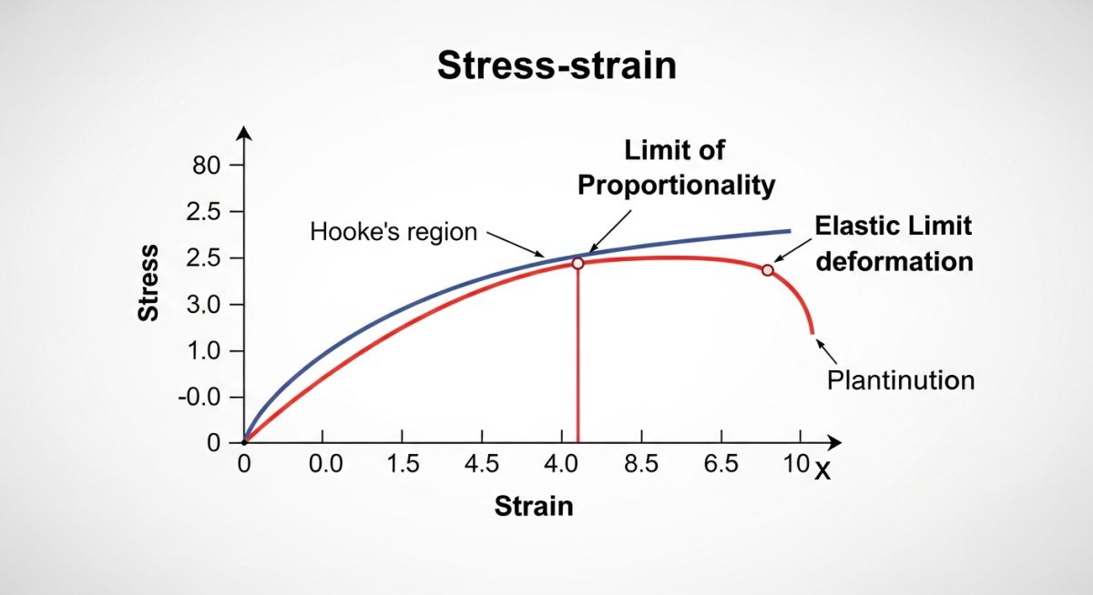
The graph is divided into several critical zones:
- Proportional Limit (Point A): This is the absolute boundary of Hooke’s Law. Up to this point, the relationship between stress and strain is a perfectly straight line. The slope of this line is equal to Young’s Modulus (E).
- Elastic Limit (Point B): Beyond Point A but up to Point B, the material will still return to its original shape when the load is removed. However, the relationship is no longer perfectly linear.
- Yield Strength (Point C): Beyond the elastic limit, the material enters the plastic region. Permanent, irreversible deformation occurs here.
- Ultimate Tensile Strength (Point D): The maximum stress the material can withstand before necking begins.
- Fracture Point (Point E): The physical rupture of the material.
Applications of Hooke’s Law
Elasticity Engineering Applications: This physical law is applied in the design of spring hangers, pressure vessel expansion joints, and structural steel frames. It enables precise calculation of thermal expansion stresses and structural load distributions.
In industrial plant design, we apply this linear relationship daily. Some of the most common applications include:
- Variable Spring Hangers: Used to support piping systems that undergo vertical thermal displacement. The spring constant (k) is selected to balance the piping weight while allowing controlled movement.
- Bellows and Expansion Joints: Designed with specific axial, lateral, and angular spring rates to absorb thermal expansion without transferring excessive loads to sensitive equipment like pumps and turbines.
- Structural Steel Design: Ensuring that steel columns, beams, and pipe racks remain well within their elastic limits under wind, seismic, and dead loads.
- Torque Wrenches and Calibration Tools: Utilizing calibrated elastic elements to measure applied force and torque during flange bolt tightening.
Limitations of Hooke’s Law
Elastic Limit Boundaries: This mechanical law is restricted to the linear elastic region of materials and fails once plastic deformation begins. It cannot predict material behavior beyond the proportional limit or under high-temperature creep conditions.
While incredibly useful, Hooke’s Law is not a universal law of physics; it is an empirical approximation. Its limitations include:
- Plastic Deformation: Once a material is stressed beyond its proportional limit, Hooke’s Law is no longer valid, and permanent deformation occurs.
- Temperature Sensitivity: At elevated temperatures, materials undergo creep (slow, progressive plastic deformation under constant stress), rendering linear elastic calculations inaccurate over time.
- Anisotropic Materials: Materials like composites, wood, or certain cast metals do not exhibit uniform elastic properties in all directions, requiring complex tensor mathematics rather than simple linear equations.
- Dynamic Loading and Fatigue: Under high-frequency cyclic loading, materials can fail due to fatigue at stress levels far below the proportional limit.
Performing Hooke’s Law Calculations
Elastic Deformation Calculations: This engineering procedure involves calculating spring forces, material stresses, and structural displacements using linear elasticity equations. It provides the quantitative basis for verifying compliance with international design codes.
Example Calculation 1: Sizing a Variable Spring Hanger
Let’s say we have a hot steam line supported by a variable spring hanger.
- Operating Load (Hot Load) = 22,000 N
- Thermal Travel (Upward displacement, x) = 15 mm
- Selected Spring Constant (k) = 120 N/mm
We need to calculate the Cold Load (Preset Load) and verify that the variability does not exceed the standard 25% limit specified by MSS SP-58.
Since the piping moves upward by 15 mm from cold to hot, the spring will decompress (extend) as the pipe heats up. Therefore, the spring must be compressed more in the cold state.
Now, let’s calculate the spring variability:
Since 8.18% is well below the 25% limit, this spring selection is highly acceptable for our piping system.
Example Calculation 2: Stress-Strain on a Carbon Steel Pipe
Consider an ASTM A106 Grade B carbon steel pipe subjected to an axial tensile load.
- Young’s Modulus (E) at 20°C = 203,000 MPa
- Measured Axial Strain (ε) = 0.0005 (dimensionless)
We need to calculate the resulting axial stress (σ) and verify if it remains within the elastic region (Yield Strength of A106-B is 240 MPa).
Since 101.5 MPa is significantly lower than the yield strength of 240 MPa, the material is operating safely within its linear elastic region, confirming that Hooke’s Law is fully valid for this operational state.
The table below provides the elastic properties of common industrial piping materials at ambient temperature (20°C). These values are critical inputs for any linear elastic stress analysis.
| Material Specification | Young’s Modulus (GPa) | Yield Strength (MPa) | Poisson’s Ratio | ASME Code Reference |
|---|---|---|---|---|
| ASTM A106 Grade B | 203 | 240 | 0.30 | ASME B31.3 Table A-1 |
| ASTM A312 TP304 | 193 | 205 | 0.29 | ASME B31.3 Table A-1 |
| ASTM A335 Grade P11 | 205 | 205 | 0.30 | ASME B31.3 Table A-1 |
| ASTM B165 (Monel 400) | 179 | 170 | 0.32 | ASME B31.3 Table A-1 |
This matrix maps the core physical entities, structural acronyms, and standard references associated with linear elasticity and piping design.
| Physical Entity | Acronym / Symbol | Primary Unit (SI) | Governing Standard | Application Scope |
|---|---|---|---|---|
| Modulus of Elasticity | E (Young’s Modulus) | GPa or MPa | ASTM E111 | Determining material stiffness and elastic deformation limits. |
| Spring Rate / Constant | k | N/mm or N/m | MSS SP-58 | Sizing variable and constant spring hangers for piping supports. |
| Allowable Stress Range | S_A | MPa | ASME B31.3 Chapter II | Evaluating thermal expansion fatigue limits in piping systems. |
| Poisson’s Ratio | ν (Nu) | Dimensionless | ASTM E132 | Calculating lateral strain resulting from axial stress. |
Verification Checklist for Hooke’s Law
Elastic Design Checklist: This verification protocol ensures that piping systems and structural supports operate strictly within their linear elastic limits. It prevents permanent plastic deformation and catastrophic structural failures during plant operations.
Before signing off on any piping stress analysis or structural design, field engineers must verify that the physical installation matches the design assumptions of linear elasticity. Use this checklist during your next walkdown:
Field Verification Checkpoints
-
Verify Spring Hanger Travel: Ensure that the actual cold-to-hot travel of all variable spring hangers matches the calculated displacement (x) from the stress report.
-
Check for Plastic Deformation: Inspect highly stressed piping elbows and structural connections for signs of yielding, paint flaking, or permanent distortion.
-
Confirm Temperature Derating: Double-check that the Young’s Modulus used in the stress calculations matches the actual operating temperature of the line per ASME B31.3.
-
Inspect Expansion Bellows: Ensure that bellows are not compressed beyond their maximum rated elastic limit during cold installation.
-
Validate Support Clearances: Confirm that pipe guides and anchors allow the calculated thermal expansion displacement without binding or causing localized over-stress.
Field Case Study: Real-World Application
Piping Stress Case Study: This field analysis documents the resolution of a critical spring hanger failure in a high-temperature steam line. It demonstrates the practical application of linear elasticity principles to restore system integrity.
The Problem: Over-stressed Steam Line Bypass
At a combined cycle power plant, a 12-inch high-pressure steam bypass line operating at 480°C was experiencing severe vibration and visible sagging near a turbine inlet. The original design utilized rigid rod hangers. During thermal expansion, the pipe expanded upward, lifting off the rigid supports and transferring its entire dead weight to the turbine nozzle. This exceeded the allowable nozzle loads specified by API 611, risking a catastrophic casing crack.
The Solution: Applying Hooke’s Law
I was brought in to redesign the support system. Using CAESAR II, we modeled the thermal displacement of the line, which showed an upward vertical movement of 18 mm at the critical support location.
Using Hooke’s Law (F = -kx), we replaced the rigid rod hanger with a variable spring hanger. We selected a spring with a spring constant (k) of 80 N/mm to balance the operating load of 14,000 N. The new design successfully absorbed the 18 mm of thermal travel while maintaining a stable supporting force, reducing the turbine nozzle load by 85% and keeping the system safely within its elastic limits.
This case highlights why understanding the linear elastic range of materials and supports is vital. A simple rigid support can turn a flexible piping system into a destructive lever if thermal expansion is not properly managed using elastic design principles.
Frequently Asked Engineering Questions
Elasticity FAQ Guide: This technical reference addresses common queries regarding the application, limits, and mathematical formulations of linear elasticity. It provides clear, code-compliant answers for practicing piping and structural engineers.
What is the difference between the proportional limit and the elastic limit?
Why is Hooke’s Law written with a negative sign in F = -kx?
How does temperature affect Hooke’s Law in piping design?
Can Hooke’s Law be applied to rubber and elastomers?
What is the relationship between Young’s Modulus and spring stiffness?
What happens if a piping system is stressed beyond Hooke’s Law limits?
===

📚 Recommended Resources: Hooke\'s Law
Related posts:
![Understanding the GRE Design Envelope for Safe Piping Operations]()
Understanding the GRE Design Envelope for Safe Piping Operations
![Understanding the Types of Fractional Distillation Process in Refining]()
Understanding the Types of Fractional Distillation Process in Refining
![Optimizing Extractive Distillation for Aromatics Separation in Petrochemical Plants]()
Optimizing Extractive Distillation for Aromatics Separation in Petrochemical Plants
![How to Select Bolting Materials for Piping Engineering Applications]()
How to Select Bolting Materials for Piping Engineering Applications
![Industrial metallic piping network with stainless steel pipes and valves in a processing plant.]()
What is Metallic Piping: Types, Advantages, Applications, and ASTM Standards
![Industrial gas processing facility comparing cryogenic LNG storage tanks and pressurized LPG bullet tanks.]()
What are the Differences Between LNG and LPG?