Table of Contents
What Is Modal Analysis? Caesar II Piping Modal Analysis Steps
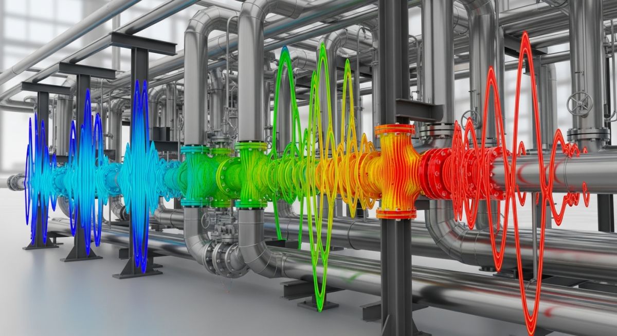
In my 20+ years of piping stress analysis, I have seen beautifully designed systems shake themselves to pieces within hours of commissioning. The culprit is almost always resonance—a phenomenon where the operating frequency of reciprocating compressors, pumps, or fluid transients matches the natural frequency of the piping system. When this happens, displacement amplitudes multiply exponentially, leading to rapid fatigue failure at branch connections and support liftoff.
To prevent these catastrophic field failures, we rely on dynamic simulation. This guide walks you through the fundamental physics of modal behavior and provides the exact, step-by-step engineering workflow I use to execute a successful dynamic analysis using Hexagon’s Caesar II software.
Key Engineering Takeaways
- Understand the mathematical formulation of the mass-stiffness dynamic equation.
- Learn how to configure the Caesar II dynamic input processor for modal extraction.
- Identify critical excitation frequencies from mechanical equipment like reciprocating pumps.
- Master the interpretation of mass participation factors and mode shapes.
- Implement effective structural modifications to shift natural frequencies out of danger zones.
Understanding Caesar II Piping Modal Analysis and Dynamic Behavior
[Piping Dynamic Behavior]: The structural response of a piping network to time-varying loads, governed by mass distribution, stiffness matrices, and boundary conditions as defined in ASME B31.3 Appendix P.
Before clicking buttons in Caesar II, we must understand the underlying mathematics. A piping system is a continuous structure with infinite degrees of freedom (DOF). In finite element analysis (FEA), Caesar II discretizes this continuous system into a finite number of beam elements. The dynamic behavior of this multi-degree-of-freedom (MDOF) system is governed by the classical equation of motion:
Where:
• [M] is the global mass matrix (representing the physical weight of the pipe, fluid, insulation, valves, and flanges).
• [C] is the damping matrix (representing energy dissipation).
• [K] is the global stiffness matrix (representing pipe wall thickness, material elasticity, and support constraints).
• {F(t)} is the time-dependent external force vector.
For free, undamped vibration (which is the basis of modal analysis), we set the damping matrix [C] and the external force vector {F(t)} to zero. This simplifies our equation to:
Assuming a harmonic solution of the form x(t) = {phi} * sin(omega * t), where {phi} is the mode shape vector and omega is the natural circular frequency (radians per second), we substitute this back to yield the classic eigenvalue problem:
To find non-trivial solutions, the determinant of the matrix ([K] – omega^2 * [M]) must equal zero. Solving this determinant yields the eigenvalues (natural frequencies) and the corresponding eigenvectors (mode shapes).
Why Modal Analysis Is the Foundation of All Dynamics
Modal analysis is not just an academic exercise; it is the prerequisite for every advanced dynamic analysis. You cannot run a spectrum analysis (for seismic or water hammer events) or a time-history analysis (for slug flow or relief valve discharge) without first extracting the system’s modes. The modal extraction tells us:
- The Natural Frequencies: Which frequencies will cause the system to resonate.
- The Mode Shapes: How the piping will physically deform at each natural frequency.
- Mass Participation Factors: Which modes contain the most kinetic energy and are therefore most susceptible to excitation by external forces.
Step-by-Step Caesar II Piping Modal Analysis Execution
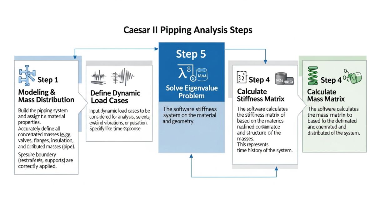
To perform a rigorous dynamic extraction in Caesar II, follow this structured engineering workflow:
- Build and Error-Check the Static Model: Ensure your piping geometry, wall thicknesses, corrosion allowances, insulation, and fluid densities are accurately defined. Run a static analysis first to verify that there are no disconnected nodes, extreme displacements, or support liftoffs under operating conditions.
- Access the Dynamic Input Processor: From the Caesar II main menu, select Analysis > Dynamics. This opens the dynamic input interface, which references your active static piping model.
- Define the Mass Model: In the Control Parameters tab, select your mass model type. I highly recommend using the Lumped Mass model for standard piping. Ensure that the software is configured to include the mass of the fluid, insulation, and cladding. If you have heavy inline components like control valve stations or strainers, verify that their weights are modeled as concentrated masses at their respective center of gravity nodes.
-
Configure the Modal Extraction Parameters:
- Select the extraction method: Lanczos is the default and most efficient solver for large piping networks.
- Set the Frequency Cutoff: For most industrial piping systems, a cutoff frequency of 33 Hz (the rigid threshold) is standard. However, for high-frequency acoustic excitation or reciprocating compressor piping, increase this cutoff to 100 Hz or higher.
- Specify the number of modes to extract. Always request more modes than you think you need (e.g., 30 to 50 modes) to ensure you capture at least 90% cumulative mass participation in all three orthogonal directions.
- Define Dynamic Constraints and Boundary Conditions: Ensure that your supports are modeled correctly for dynamic behavior. For example, a simple pipe hanger provides vertical support in statics but offers zero lateral or axial restraint during dynamic shaking. If you have snubbers or spring hangers, ensure their dynamic stiffness values are correctly populated.
- Run the Dynamic Solver: Click the Run icon to execute the eigensolver. The software will build the global mass and stiffness matrices, perform the Sturm sequence check, and extract the requested eigenvalues and eigenvectors.
Excitation Frequency Thresholds and Guidelines
[Excitation Frequency Thresholds]: The critical frequency ranges associated with mechanical equipment and fluid transients that must be avoided to prevent resonance in piping systems.
To design a dynamically stable piping system, we must ensure that the natural frequencies of our piping do not coincide with the excitation frequencies of connected equipment. The table below outlines typical excitation sources, their frequency ranges, and the recommended design targets.
| Excitation Source | Typical Frequency Range (Hz) | Target Piping Natural Frequency (Hz) | Mitigation & Design Strategy |
|---|---|---|---|
| Reciprocating Compressors | 5 to 120 Hz (1x, 2x, and higher harmonics) | > 33 Hz (or at least 20% separation from harmonics) | Install rigid, heavy-duty supports; minimize overhangs; design pulsation dampeners per API 618. |
| Centrifugal Pumps (Vane Pass) | 50 to 300 Hz (RPM x Number of Impeller Vanes) | Avoid vane pass frequency by +/- 20% | Use stiff, short-span supports near pump nozzles; avoid flexible bellows if possible. |
| Wind-Induced Vortex Shedding | 0.5 to 5 Hz (Low frequency, high amplitude) | > 5 Hz for tall vertical columns/piping | Add helical strakes or structural guide supports to break up vortex formation. |
| Acoustic Induced Vibration (AIV) | 500 to 2000 Hz (High frequency, low displacement) | N/A (Governed by shell mode excitation) | Increase pipe wall thickness; use wrap-around reinforcing pads at branch connections. |
Technical Mapping & Specifications Matrix
This matrix maps the core physical parameters, mathematical entities, and standard references used during a Caesar II dynamic simulation.
| Entity / Parameter | Technical Definition | Physical Unit | Standard Reference |
|---|---|---|---|
| Mass Matrix [M] | Representation of the distributed and concentrated mass of the piping system. | kg (or lbs) | ASME B31.3 Appendix P |
| Stiffness Matrix [K] | Representation of the structural resistance to deformation based on geometry and material. | N/m (or lb/in) | ASME B31.3 / ASME B31.1 |
| Mass Participation Factor | Measure of the amount of system mass active in a specific mode shape direction. | Dimensionless (Percentage) | ASME Section III Division 1 |
| Rigid Cutoff Frequency | The frequency beyond which structural modes do not contribute significantly to dynamic response. | Hz (Hertz) | US NRC Regulatory Guide 1.92 |
Pre-Analysis Checklist for Caesar II Piping Modal Analysis
[Pre-Analysis Verification]: The systematic validation of piping model geometry, support configurations, and mass distributions prior to executing dynamic solvers in Caesar II.
Before running your dynamic solver, use this checklist to ensure your model represents physical reality. A minor error in mass or boundary conditions will yield incorrect natural frequencies, rendering your dynamic analysis useless.
Dynamic Model Validation Steps
Ensure the fluid density is active in the dynamic input. For gas lines, verify that the liquid-fill case is modeled if hydrotesting dynamic checks are required.
Verify that all heavy inline valves, actuators, and flanges have their weights modeled as concentrated masses at their exact center of gravity. Do not let the software treat them as plain pipe.
Dynamic solvers linearize the system. If you have supports with large gaps, decide whether they are active or inactive during dynamic shaking. Friction coefficients should generally be set to zero for conservative dynamic results.
Ensure that equipment nozzles (e.g., pump or vessel connections) are modeled with realistic local stiffness values rather than as infinitely rigid anchors. Rigid anchors artificially inflate natural frequencies.
Verify that the extracted modes achieve at least 90% cumulative mass participation in the X, Y, and Z directions. If not, increase the number of requested modes or raise the cutoff frequency.
Field Case Study: Real-World Application
The Problem: Severe Vibration in a Gas Processing Plant
During the commissioning of a natural gas processing facility, a 12-inch reciprocating compressor discharge line experienced severe, visible shaking. Vibration measurements showed peak-to-peak displacement amplitudes exceeding 15 mm/s RMS at the first elbow downstream of the pulsation dampener. The plant operator was forced to throttle the compressor, reducing production by 30% to prevent a fatigue blowout. The original design team had only performed static stress analysis, completely omitting dynamic modal checks.
The Solution: Caesar II Modal Extraction and Structural Tuning
I was brought in to resolve the issue. First, we built a high-fidelity Caesar II model of the discharge line, including the concentrated mass of the control valves and the exact stiffness of the existing pipe guides.
Our initial modal extraction revealed a dominant 1st natural frequency of 14.2 Hz with a mode shape showing massive lateral displacement at the troublesome elbow. The compressor operated at 850 RPM, which translates to a fundamental excitation frequency of 14.17 Hz (850 / 60). The system was in near-perfect resonance!
To solve this, we designed a rigid structural strut support (axial restraint) at the elbow to stiffen the system. We re-ran the Caesar II modal analysis with the new support. The 1st natural frequency shifted from 14.2 Hz to 28.4 Hz, safely exceeding the compressor’s 1x operating frequency and providing a 100% separation margin.
Direct Recommendation: Never rely solely on static stress analysis for piping connected to reciprocating machinery. Always perform a modal analysis during the detailed engineering phase. If you identify a natural frequency within 20% of the equipment’s operating speed, add rigid supports or struts to shift the frequency upward. Stiffening the system is almost always more effective than trying to damp the vibration after the fact.
Frequently Asked Engineering Questions
[Modal Analysis FAQs]: A curated compilation of technical answers addressing common challenges, solver settings, and code compliance in piping dynamic analysis.
1. What is the difference between a static analysis and a modal analysis in Caesar II?
2. Why is 33 Hz commonly used as the cutoff frequency in modal extraction?
3. How do I resolve a warning about low mass participation in Caesar II?
4. Can I use spring hangers to mitigate piping vibration issues?
5. How does fluid density affect the natural frequencies of a piping system?
6. Which design codes govern dynamic and modal analysis for process piping?
===FAQ_BLOCK===
Complete Course on
Piping Engineering
Check Now
Key Features
- 125+ Hours Content
- 500+ Recorded Lectures
- 20+ Years Exp.
- Lifetime Access
Coverage
- Codes & Standards
- Layouts & Design
- Material Eng.
- Stress Analysis

📚 Recommended Resources: Caesar II piping modal analysis
Read these Guides
🎓 Advanced Training
🎥 Watch Tutorials

Related posts:
![Infographic flowchart of the GRP GRE FRP piping stress analysis workflow in START-PROF.]()
Rigid Struts: Definition, Applications, and Modeling in Caesar II
![3D stress analysis model of GRP piping system in START-PROF software showing stress distribution.]()
Stress Analysis of GRP / GRE / FRP Piping using START-PROF
![Industrial centrifugal pump installed on a concrete foundation with precision piping and alignment.]()
How to Use a Pump Installation Checklist for Maximum Reliability
![3D Caesar II pipe stress analysis model of a centrifugal pump piping system showing stress distribution.]()
Pump-Piping Alignment Caesar II Stress Analysis Methodology
![3D render of a structural steel cross-bracing connection with a gusset plate.]()
Mastering Steel Connections with a Cross-Bracing Design Example
![Industrial engineer checking shaft alignment on a centrifugal pump during commissioning.]()
How to Use a Pump Commissioning Checklist for Start-Up