Mastering Bernoulli’s Equation and Principle in Piping Systems
In my 20 years of designing and troubleshooting industrial piping networks, I have seen many young engineers treat fluid dynamics as a set of abstract formulas. But when you are standing on a refinery deck, listening to the violent rattle of a cavitating control valve or watching a pump struggle to meet its head requirements, those formulas become your only shield. Bernoulli’s principle is not just a textbook derivation; it is the absolute foundation of how we move fluids safely from point A to point B.
Whether you are sizing a Venturi flowmeter, calculating NPSH for a critical process pump, or analyzing pressure drops across complex manifolds, you must master the balance between kinetic energy, potential energy, and pressure energy. In this guide, I will walk you through the practical mechanics of Bernoulli’s equation, strip away the academic fluff, and show you how to apply these principles directly to real-world piping design.
What You Will Master in This Guide:
- The rigorous mathematical derivation of Bernoulli’s equation from Euler’s equation of motion.
- How to apply energy conservation principles to real-world, compressible, and viscous fluid flows.
- Practical engineering calculations for Venturi meters, orifice plates, and piping hydraulic profiles.
- A field-tested checklist to verify fluid assumptions and prevent catastrophic cavitation on site.
How Do We Derive Bernoulli’s Equation?
Bernoulli’s Equation Derivation: The mathematical integration of Euler’s equation of motion along a streamline under steady-state conditions, translating Newton’s second law into an energy conservation statement for ideal fluids.
To truly understand the limits of Bernoulli’s equation, we must look at how it is built. We start with Euler’s equation of motion for an inviscid, frictionless fluid along a streamline. Consider a small fluid element of length (ds) and cross-sectional area (dA) moving along a streamline. The forces acting on this element are the pressure forces on both ends and the component of gravity acting along the direction of motion.
Applying Newton’s second law ((F = ma)) along the streamline direction (s), we write:
Where (theta) is the angle between the streamline and the vertical gravity vector, meaning (cos(theta) = dz/ds). The acceleration along the streamline (a_s) for steady flow is given by the convective acceleration (v * (dv/ds)). Substituting these terms and simplifying the equation yields Euler’s equation of motion:
Integrating this differential equation along the streamline with respect to (s) for an incompressible fluid (where density (rho) is constant) gives us the classic Bernoulli equation:
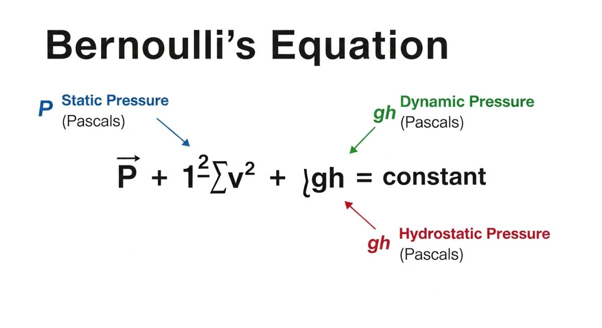
In my design work, I prefer to express this in terms of “head” (meters or feet of fluid column) by dividing the entire equation by (rho * g). This format is highly practical for pump sizing and hydraulic modeling:
Where:
- Static Pressure Head ((P / rho g)): Represents the potential energy stored in the fluid due to static pressure.
- Velocity Head ((v^2 / 2g)): Represents the kinetic energy of the fluid per unit weight.
- Elevation Head ((z)): Represents the potential energy due to the height above a reference datum.
- Total Head ((H)): The constant sum of energy along any streamline in an ideal fluid.
In real-world process plants, there is no such thing as a frictionless fluid. Every pipe wall, elbow, valve, and tee introduces shear stress and turbulence, converting mechanical energy into non-recoverable thermal energy. If you apply the ideal Bernoulli equation to a long-distance transfer line without adding a friction loss term ((h_f)), your downstream pressure calculations will be dangerously high, leading to undersized pumps and system starvation. Always use the modified engineering energy equation:
Real-World Flow Measurement: The Venturi Tube
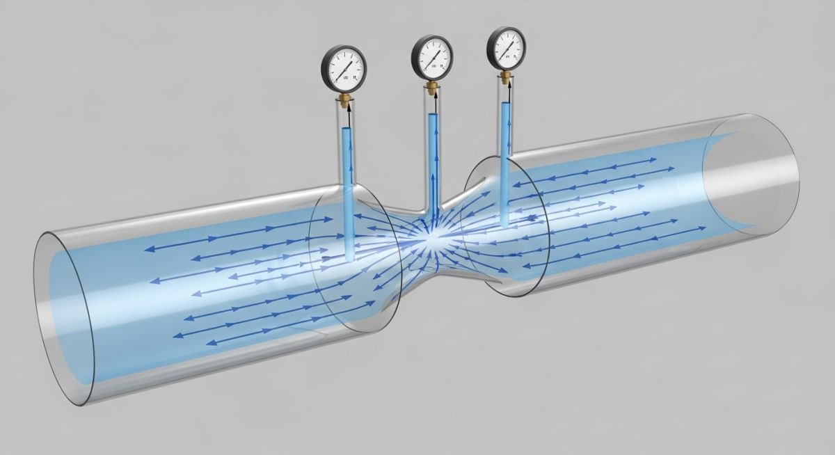
One of the most elegant applications of Bernoulli’s principle is the Venturi tube, governed by ASME MFC-3M standards. By constricting the flow area from a diameter (D_1) to a throat diameter (D_2), the fluid velocity must increase to satisfy the continuity equation ((A_1 v_1 = A_2 v_2)).
According to Bernoulli, this localized increase in kinetic energy causes a corresponding drop in static pressure at the throat. By measuring this differential pressure ((Delta P = P_1 – P_2)), we can calculate the precise volumetric flow rate using:
Where (C_d) is the discharge coefficient (typically 0.98 for a well-machined Venturi) and (beta) is the diameter ratio ((D_2 / D_1)).
Fluid Velocity and Pressure Drop Reference
Fluid Velocity Reference Data: Standardized operational parameters mapping volumetric flow rates to differential pressure drops across varying pipe schedules to prevent cavitation and erosion.
In my practice, I use standardized velocity limits to balance piping cost against energy loss. High velocities reduce pipe size but cause massive pressure drops and erosion. Low velocities require oversized, expensive piping. The table below shows typical design parameters for water at 20°C flowing through Schedule 40 carbon steel pipes, calculated using the Darcy-Weisbach and Bernoulli equations.
| Nominal Pipe Size (NPS) | Flow Rate (m³/h) | Mean Velocity (m/s) | Velocity Head (m of fluid) | Pressure Drop (bar/100m) | Flow Regime (Reynolds No.) |
|---|---|---|---|---|---|
| 2″ (DN 50) | 15.0 | 2.05 | 0.21 | 1.85 | 1.1 x 10⁵ (Turbulent) |
| 4″ (DN 100) | 60.0 | 2.12 | 0.23 | 0.78 | 2.2 x 10⁵ (Turbulent) |
| 6″ (DN 150) | 140.0 | 2.18 | 0.24 | 0.45 | 3.4 x 10⁵ (Turbulent) |
| 8″ (DN 200) | 250.0 | 2.22 | 0.25 | 0.31 | 4.6 x 10⁵ (Turbulent) |
To ensure compliance with global engineering standards, the following matrix maps the core physical entities of fluid dynamics to their corresponding industry codes and physical parameters.
| Technical Entity | Acronym | Primary Physical Parameter | Governing Standard Reference |
|---|---|---|---|
| Net Positive Suction Head | NPSH | Absolute Static Pressure (m) | ASME B73.1 / API 610 |
| Differential Pressure Flowmeters | DP Flow | Pressure Drop ((Delta P)) | ISO 5167 / ASME MFC-3M |
| Piping Hydraulic Design | PHD | Friction Loss Head ((h_f)) | ASME B31.3 Process Piping |
| Control Valve Sizing | CVS | Flow Coefficient ((C_v)) | ISA-75.01.01 / IEC 60534 |
How to Verify Bernoulli Assumptions on Site?
Bernoulli Field Verification Checklist: A systematic quality control protocol designed to validate steady-state flow assumptions, piping geometry constraints, and instrumentation calibration before hydraulic testing.
Before you sign off on a hydraulic design or start up a newly installed process line, you must verify that the physical installation matches the mathematical assumptions of your fluid models. Use this checklist during your next walkdown:
Pre-Commissioning Hydraulic Checklist
-
Verify Steady-State Flow Conditions: Ensure the system is not operating under severe transient cycles or pulsating flows (e.g., downstream of reciprocating pumps without pulsation dampeners), which violate the steady-state assumption of Bernoulli.
-
Check Straight Pipe Runs for DP Meters: Confirm that Venturi tubes or orifice plates have at least 10 diameters of straight, unobstructed pipe upstream and 5 diameters downstream to prevent velocity profile distortion, as required by ISO 5167.
-
Validate Elevation Reference Datums: Double-check that all pressure transmitter elevations match the isometric drawings. A 1-meter error in elevation head calculation translates to a 9.8 kPa static pressure discrepancy for water.
-
Inspect for High-Point Air Pockets: Ensure all high points in liquid lines are equipped with functional air release valves. Trapped air pockets restrict the flow area, causing localized velocity increases and unexpected pressure drops.
-
Confirm Fluid Phase Stability: Verify that the minimum static pressure at any point in the system (especially at control valve throats or pump suctions) remains safely above the fluid’s vapor pressure at operating temperature to prevent cavitation.
Field Case Study: Real-World Application
The Problem: Cavitation and Vibration in a Cooling Water Return Line
At a petrochemical plant in Singapore, a 12-inch cooling water return line was experiencing severe, localized vibration and a loud crackling noise resembling gravel flowing through the pipe. The issue occurred immediately downstream of a control valve that throttled the return flow to a cooling tower.
The plant engineers suspected valve trim failure, but my physical walkdown and hydraulic analysis revealed a different story. The control valve was located at a high point in the piping layout, approximately 8 meters above the cooling tower basin. Because the valve was throttling the flow, the localized velocity head ((v^2 / 2g)) increased dramatically at the valve throat, causing the static pressure head ((P / rho g)) to drop below the vapor pressure of the water (which was 3.17 kPa absolute at the 25°C operating temperature). This triggered flash vaporization, followed by violent bubble collapse (cavitation) as the pressure recovered downstream.
The Solution: Applying Bernoulli to Restore Static Pressure
Instead of purchasing an expensive multi-stage control valve, I redesigned the piping hydraulics using Bernoulli’s energy conservation principles. We implemented two key modifications:
- We relocated the control valve from the high-point elevation down to ground level, immediately before the cooling tower inlet. This increased the static elevation head ((z)) at the valve inlet by 8 meters, which directly translated to an additional 78.5 kPa of static pressure, keeping the fluid well above its vapor pressure.
- We installed a concentric reducer downstream of the valve to gradually transition the velocity back to the main line speed, minimizing turbulent energy loss and preventing sudden pressure recovery shocks.
The result? The cavitation noise and vibration were completely eliminated. The system has now run for over five years without a single valve trim replacement or pipe wall thinning issue.
Frequently Asked Engineering Questions
Can Bernoulli’s equation be applied to compressible gases?
What is the difference between static pressure, dynamic pressure, and total pressure?
How does pipe roughness affect Bernoulli calculations?
Why does pressure drop when fluid velocity increases in a restriction?
How do you account for elevation changes in a closed-loop system?
What is the relationship between Bernoulli’s principle and cavitation?

📚 Recommended Resources: Bernoulli\'s Equation and Principle
Read these Guides
Related posts:
![Technical infographic showing the workflow of flood risk assessment for data centres, including hydrological inputs and mitigation strategies.]()
Flood Risk Assessment for Data Centres: Engineering Design Guide
![Isometric engineering rendering of a data centre campus featuring flood protection barriers and elevated utility infrastructure for disaster resilience.]()
Flood Protection Level Selection for Mission-Critical Data Centre Infrastructure
![Cross-section diagram of a data centre foundation showing soil strata, pile foundations, and groundwater monitoring wells for geotechnical analysis.]()
Geotechnical Requirements for Data Centres: A Structural Engineering Guide
![Civil 3D interface showing a 3D site grading model with color-coded cut and fill zones for earthwork optimization.]()
Optimizing Cut and Fill Operations Using Civil 3D and GIS
![3D digital terrain model showing site grading, flood protection levels, and cut-fill zones for industrial infrastructure development.]()
Establishing FPL and Estimating Cut Fill Quantities for Site Grading
![3D engineering model showing cut and fill optimization for industrial site grading and earthwork balancing.]()
Cut and Fill Optimization: 8 Engineering Studies for Site Grading