Table of Contents
What is Time History Analysis? Steps with CAESAR II Example
In my 20-plus years of resolving piping stress failures on high-pressure steam lines and petrochemical facilities, I have seen static analysis fall short when transient forces strike. When a main steam isolation valve slams shut in milliseconds, or a slug of liquid crashes through an overhead vapor line, static approximations simply cannot capture the true physical reality. That is where a rigorous dynamic simulation becomes your primary line of defense.
I wrote this guide to demystify the exact mathematical and practical steps required to execute a successful dynamic simulation. We will walk through the core physics, look at how to configure the dynamic solver in CAESAR II, and establish a clear workflow that you can apply directly to your next high-risk piping project.
Key Engineering Takeaways
- Understand the physical triggers that demand a full transient dynamic evaluation over static approximations.
- Master the step-by-step translation of fluid transient force-time profiles into CAESAR II.
- Learn how to configure modal extraction, integration time steps, and damping ratios to prevent numerical divergence.
- Compare the structural realism of time-history methods against response spectrum profiles.
Complete Course on
Piping Engineering
Check Now
Key Features
- 125+ Hours Content
- 500+ Recorded Lectures
- 20+ Years Exp.
- Lifetime Access
Coverage
- Codes & Standards
- Layouts & Design
- Material Eng.
- Stress Analysis
Reason for Dynamic Time History Analysis
Dynamic Piping Response: The evaluation of transient forces over discrete time steps ensures that high-velocity fluid events do not cause catastrophic structural resonance or yield-strength failures.
When a fluid velocity change occurs rapidly, the piping system experiences an instantaneous unbalanced force. If you try to analyze this using a static equivalent multiplier (such as applying a generic 2.0 DLF factor to a static load case), you risk either over-designing the support structure or missing critical localized stress peaks.
The physical response of the piping system is governed by Duhamel’s Duhamel integral, which maps the system’s displacement response over time:
Where:
• m is the modal mass of the system.
• ωn is the natural undamped frequency.
• ωd is the damped natural frequency.
• ζ is the structural damping ratio.
• F(τ) is the time-varying force vector.
Without solving this time-dependent relationship, you cannot accurately predict the phase relationships between different spans of piping. One loop might be moving left while another moves right, creating massive bending moments at intermediate tees that a static analysis completely ignores.
In my field audits, I frequently find stress packages where engineers applied a default Dynamic Load Factor (DLF) of 2.0 in a static run to simulate water hammer. This assumption is highly dangerous. If the fluid transient rise time aligns perfectly with the first natural frequency of a long piping span, the actual DLF can exceed 2.0 due to resonance, leading to unexpected support failure or flange leakage. Always run a dynamic verification when valve closure times are under 100 milliseconds.
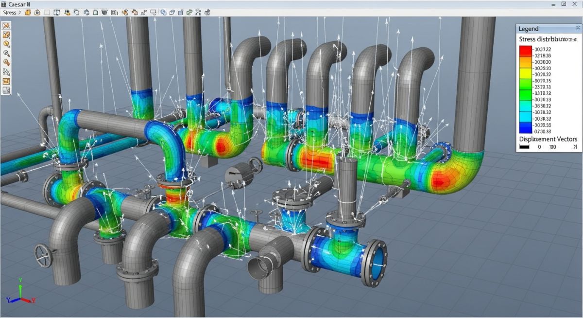
Time History Analysis Example using Caesar II
CAESAR II Dynamic Modeling: The execution of a step-by-step transient simulation in CAESAR II translates time-force profiles into real-time displacement, velocity, and stress profiles.
To illustrate the workflow, let us look at a common industrial scenario: a high-pressure boiler feedwater line experiencing a sudden pump trip. The resulting pressure wave generates transient forces at every change in piping direction. Here is how we translate this physical event into a mathematical model inside CAESAR II.
1. Modification in the Static Model
Static Model Adjustments: The conversion of a static piping model for dynamic analysis requires the refinement of support gaps, boundary conditions, and mass distribution parameters.
Before opening the dynamic module, you must ensure your static model is dynamic-ready. This means modeling actual support gaps instead of assuming rigid restraints. I always verify that the mass of insulation, inline valves, and fluid contents are precisely defined. In a dynamic run, CAESAR II converts these masses into lumped mass points at each node. If your node spacing is too wide, the program will not capture higher-frequency mode shapes. I recommend adding intermediate nodes on long, unsupported spans to ensure accurate mass distribution.
2. Defining Dynamic Loads for Time history analysis
Dynamic Load Definition: The input of transient force profiles utilizes time-history force files to simulate rapid valve closures or slug flow impacts.
To define the transient load, you must generate a force-versus-time profile. This is typically calculated using fluid transient software (like AFT Impulse) or manual water hammer equations. Once you have the force profiles for each elbow or change in direction, you import them into CAESAR II as a .force file. Each profile maps the force magnitude against time steps (typically in milliseconds). You then link these force profiles to specific node numbers where the physical impact occurs.
3. Setting up the Dynamic Control Parameters
Dynamic Control Parameters: The selection of integration time steps and modal damping ratios governs the mathematical convergence and accuracy of the dynamic solver.
This is where many engineers run into trouble. In the Dynamic Control Parameters dialog, you must specify the modal extraction limit. I recommend extracting enough modes to reach at least 90% mass participation in all three coordinate directions. Next, set your integration time step. A good rule of thumb is to set the time step to at least one-tenth of the period of the highest significant mode extracted. If your highest mode is 50 Hz (period of 0.02 seconds), your integration time step should be 0.002 seconds or smaller to prevent numerical instability.
Selecting the correct damping ratio and dynamic load factor is critical for aligning your simulation with real-world physical behavior. The table below outlines standard values based on industry research and ASME B31.3 guidelines.
| Piping System Condition | Recommended Damping Ratio (ζ) | Typical Dynamic Load Factor (DLF) | Primary Code Reference |
|---|---|---|---|
| Insulated High-Temp Steam Lines | 1.0% to 2.0% | 1.1 to 1.5 | ASME B31.1 Appendix II |
| Uninsulated Process Piping (Heavy Wall) | 2.0% to 3.0% | 1.3 to 1.8 | ASME B31.3 Chapter II |
| Cryogenic Piping with Rigid Supports | 0.5% to 1.0% | 1.5 to 2.0 | ASME B31.3 Section 301.2 |
| FRP / GRP Non-Metallic Piping | 5.0% to 10.0% | 1.0 to 1.2 | ASME NM.1 Standard |
This matrix maps the core technical entities of a dynamic simulation to their physical parameters, mathematical solvers, and corresponding compliance standards.
| Simulation Entity | Physical Parameter | Mathematical Solver Method | Standard Reference Link |
|---|---|---|---|
| Modal Extraction | Eigenvalues & Eigenvectors | Lanczos or Subspace Iteration | ASME B31.3 Appendix P |
| Time Integration | Displacement vs. Time Step | Newmark-Beta or Wilson-Theta | ASME B31.1 Section 101.5 |
| Damping Matrix | Energy Dissipation Rate | Rayleigh Damping (Alpha/Beta) | ASME Boiler & PV Code Sec III |
| Force-Time Profile | Unbalanced Transient Force | Direct Force Vector Mapping | ASME B31.3 Chapter II |
Dynamic Model QA/QC Verification Checklist
Model Validation Protocol: The systematic verification of dynamic inputs, boundary conditions, and solver parameters ensures the mathematical integrity of the simulation before finalizing support designs.
Before you rely on the stress outputs of your dynamic run to order expensive spring hangers or snubbers, you must perform a rigorous QA/QC check. In my practice, I use this checklist to catch modeling errors that could lead to non-conservative results.
Pre-Run Verification Steps
-
Mass Distribution Check: Ensure all inline valves, flanges, and heavy instruments have their actual weights modeled. Verify that the fluid density matches the operating fluid condition.
-
Support Gap Realism: Confirm that guide and limit stop gaps are modeled as actual physical dimensions rather than infinite rigid constraints.
-
Modal Mass Participation: Verify that the extracted modes achieve at least 90% mass participation in X, Y, and Z directions. If not, increase the number of requested modes.
-
Integration Time Step: Confirm that the time step is small enough to capture the highest frequency mode (typically dt ≤ 1 / (10 * f_max)).
-
Damping Ratio Alignment: Ensure the damping ratio matches the structural insulation and support type in accordance with ASME B31.3.
Field Case Study: Real-World Application
A combined-cycle power plant experienced repeated structural damage to its cooling water line supports during emergency pump shutdowns. The original design team had used a static equivalent analysis with a 2.0 DLF to design the supports. Despite this, a major transient event tore a 10-ton anchor support clean off its concrete pedestal, causing an unscheduled plant shutdown costing 150,000 per day.
I was brought in to perform a forensic dynamic evaluation. We modeled the system in CAESAR II using a full Time History Analysis. By importing the exact force-time profile generated from a hydraulic transient solver, we discovered that the pressure wave’s reflection time matched the natural frequency of the long horizontal run perfectly. This created a localized resonance that drove the actual DLF up to 3.4—far exceeding the original static design assumption of 2.0.
Using the dynamic stress profiles, we redesigned the support system by replacing two rigid guides with hydraulic snubbers and adding a targeted structural strut. The plant restarted safely, and subsequent emergency shutdowns have occurred with zero structural damage or pipe movement.
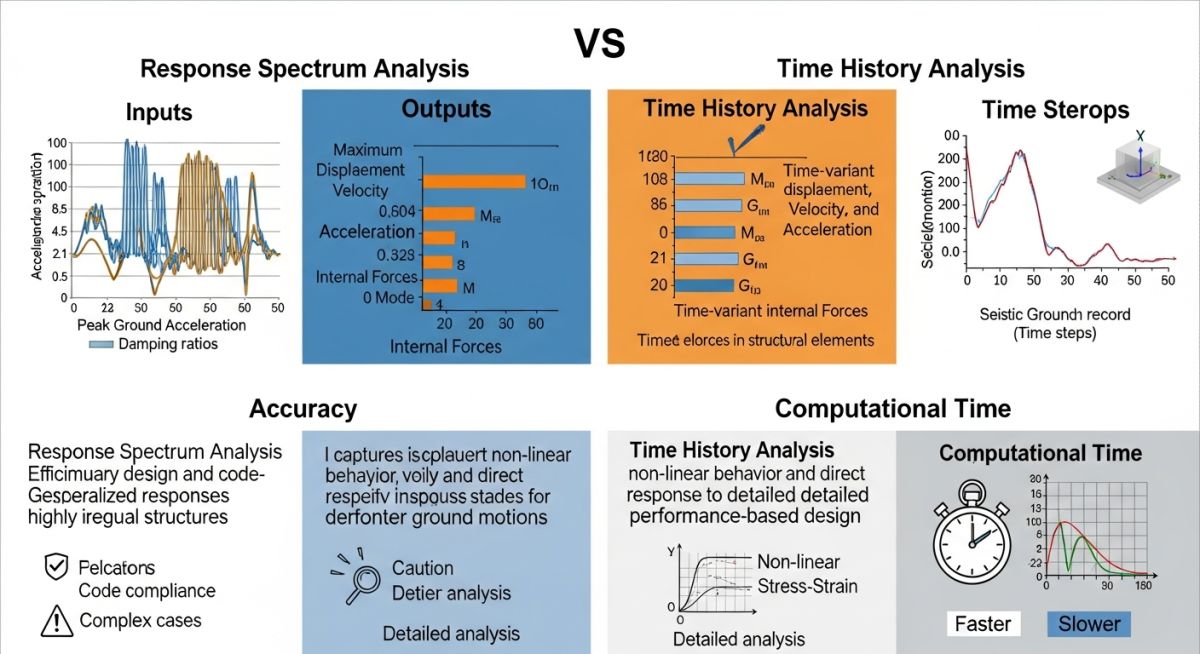
Response Spectrum vs Time History Analysis
Dynamic Analysis Comparison: The choice between response spectrum and time-history methods depends on whether the excitation is a steady-state seismic event or a highly localized transient shock.
While both methods fall under the umbrella of dynamic analysis, they serve very different purposes. Response spectrum analysis is a frequency-domain tool that calculates the maximum response of a system to a given spectrum of ground motion (like an earthquake). It is computationally efficient but does not preserve the time-phase relationship of the forces. Time History Analysis, on the other hand, is a time-domain tool that tracks the exact physical state of the system at every millisecond, making it the only viable choice for localized, non-seismic transient events like water hammer or relief valve discharge.
Frequently Asked Engineering Questions
When should I use Time History Analysis instead of Response Spectrum Analysis?
How do I determine the correct integration time step for my dynamic model?
What damping ratio should I use for a standard carbon steel steam line?
Why does CAESAR II require a static load case before running a dynamic analysis?
How do I handle non-linear supports like one-way restraints in a dynamic run?
What is the minimum mass participation required for a code-compliant dynamic run?
===EOF===

📚 Recommended Resources: Time History Analysis
Related posts:
![Industrial metallic piping network with stainless steel pipes and valves in a processing plant.]()
What is Metallic Piping: Types, Advantages, Applications, and ASTM Standards
![Industrial gas processing facility comparing cryogenic LNG storage tanks and pressurized LPG bullet tanks.]()
What are the Differences Between LNG and LPG?
![Split-screen comparison of liquid oil failing under extreme heat versus dry graphite lubricating a mechanical bearing smoothly.]()
Why Is Graphite a Better Lubricant Than Oil in Industrial Piping?
![Tall industrial distillation column tower at a chemical processing plant]()
What is a Distillation Column? Working Principles and Types
![Close-up of various metal pipe fittings with different thread types on an engineering blueprint.]()
Understanding the Different Types of Pipe Threads in Piping Systems
![A collection of different metal and plastic pipe ferrules resting on an engineering blueprint.]()
How Do Pipe Ferrules Ensure Leak-Free Industrial Piping Systems?