
K-Factor Minor Losses: The Engineering Guide to Calculation
The calculation of K-Factor Minor Losses is a fundamental requirement for hydraulic piping design, determining how fittings, valves, and junctions impact system pressure. While the Darcy-Weisbach equation handles friction, resistance coefficients define the energy dissipation caused by geometry changes in turbulent flow.
What are K-Factor Minor Losses?
K-Factor Minor Losses represent the dimensionless resistance coefficient (K) used to calculate pressure drop in pipe fittings. It is defined by the formula hL = K * (v2 / 2g), where K accounts for energy lost due to friction and flow separation in components like elbows, tees, and valves.
Engineering Knowledge Check
Question 1 of 5
Complete Course on
Piping Engineering
Check Now
Key Features
- 125+ Hours Content
- 500+ Recorded Lectures
- 20+ Years Exp.
- Lifetime Access
Coverage
- Codes & Standards
- Layouts & Design
- Material Eng.
- Stress Analysis
Fundamental Theory of K-Factor Minor Losses for Incompressible Liquids
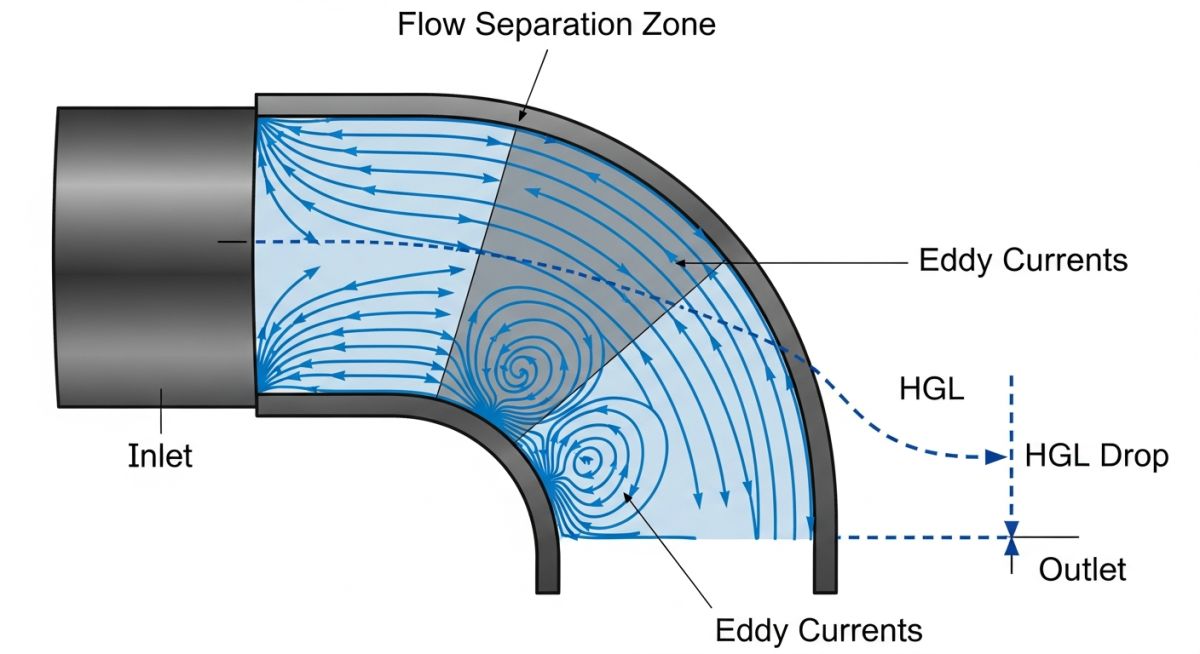
In fluid mechanics, K-Factor Minor Losses represent the energy dissipation caused by the structural geometry of a piping system. Unlike major losses, which occur along the length of a straight pipe due to wall friction, minor losses are localized phenomena. They occur at points of flow disruption such as valves, bends, and contractions. For an incompressible liquid, this loss is modeled as a reduction in total head.
The Physics of Resistance Coefficient K
The Resistance Coefficient K is a dimensionless value that correlates the velocity head of the fluid to the pressure drop. When a liquid encounters a fitting, the flow separates from the walls, creating eddies and vortices. This turbulence converts kinetic energy into thermal energy, which cannot be recovered. In accordance with ASME and ISO 12266 standards, the magnitude of this loss is directly proportional to the square of the velocity.
“While termed ‘minor’, these losses can account for more than 50 percent of the total pressure drop in complex process skids with high fitting densities.”
Industry Standards and References for K-Factor Minor Losses Calculation
Accurate engineering requires standardized data. Determining K-Factor Minor Losses relies on empirical data collected over decades. Engineers must choose the correct methodology based on the flow regime and the specific fitting geometry.
The Authority of Crane Technical Paper 410
The Crane Technical Paper 410 (TP-410) is the primary reference for Pipe Fitting Loss Coefficients. It provides the “K” values for a vast range of components, from gate valves to sudden enlargements. Most modern hydraulic modeling software packages utilize the Crane methodology as their core computational engine. Other critical references include:
- Idelchik’s Handbook of Hydraulic Resistance: Offers deep analytical data for complex Turbulent Flow Minor Losses in non-standard geometries.
- Miller’s Internal Flow Systems: Focuses on high-accuracy data for large-scale industrial ducts and piping manifolds.
- API RP 14E: Provides specific guidance for sizing and losses in offshore production platform piping.
| Fitting Type | Typical K-Value Range | Reference Standard |
|---|---|---|
| Standard 90 Elbow | 0.3 – 0.9 | Crane TP-410 |
| Globe Valve (Fully Open) | 4.0 – 10.0 | ASME B16.34 |
| Swing Check Valve | 2.0 – 2.5 | Crane TP-410 |
Calculating Resistance Coefficients for T-Junction Pipe Fittings
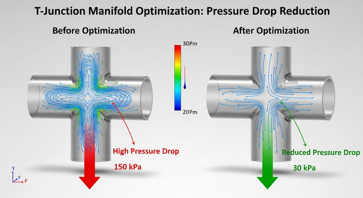
T-junctions represent one of the most complex scenarios when determining K-Factor Minor Losses. Unlike a simple elbow, a tee involves flow splitting or merging, which creates significant Turbulent Flow Minor Losses due to the impingement of fluid against the fitting wall.
Branch vs. Through-Flow Resistance
When calculating Pipe Fitting Loss Coefficients for a tee, engineers must distinguish between the “through” path and the “branch” path. The branch path typically exhibits a much higher resistance because the fluid must undergo a 90-degree change in direction, leading to a large vena contracta and secondary flow patterns.
| Flow Configuration | Flow Direction | Approximate K-Factor |
|---|---|---|
| Standard Tee | Flow-through Run | 20 ft |
| Standard Tee | Flow-through Branch | 60 ft |
The Mathematical Basis of Minor Losses
The conversion of kinetic energy into head loss is calculated using the following engineering relationship. Note that all units must be consistent (typically SI or US Customary) to ensure the Resistance Coefficient K remains dimensionless.
// Head Loss Equation for K-Factor Minor Losses
hL = K * (v2 / (2 * g))
hL = Static Head Loss (m or ft)
K = Resistance Coefficient (Dimensionless)
v = Mean Flow Velocity (m/s or ft/s)
g = Acceleration due to gravity (9.81 m/s2 or 32.2 ft/s2)
Critical Engineering Insights: Why K-Factor Minor Losses Matter in System Design
In high-velocity systems, K-Factor Minor Losses can dominate the total system resistance. If these losses are underestimated during the FEED (Front-End Engineering Design) phase, the selected pump may operate at the end of its curve, leading to cavitation, vibration, and premature seal failure.
Impact of Turbulent Flow Minor Losses
As Reynolds numbers increase, the flow becomes fully turbulent. In this regime, the Equivalent Length Method and the K-factor method become more reliable. However, engineers must be cautious with non-Newtonian fluids or laminar flow regimes, where standard Pipe Fitting Loss Coefficients from Crane TP-410 may require correction factors.
EPCLand YouTube Channel
2,500+ Videos • Daily Updates
K-Factor Minor Losses Calculator
Formula: hL = K * (v2 / (2 * g)). Standard for incompressible turbulent flow.
Case Study: Reducing K-Factor Minor Losses in a Refinery Cooling Loop
Project Data & Context
In 2026, an aging petrochemical facility faced a 15 percent deficit in cooling water flow. The system utilized a series of high-density T-junctions and globe valves. Initial analysis suggested the pump was underperforming, but a hydraulic audit revealed that K-Factor Minor Losses were significantly higher than the original design specs due to internal scaling and outdated Pipe Fitting Loss Coefficients.
- Fluid: Industrial Process Water
- System Velocity: 4.5 m/s (High Turbulence)
- Observed Pressure Drop: 1.2 bar across the manifold
Failure Analysis
The use of standard threaded tees created high Turbulent Flow Minor Losses. Each branch junction had a K-factor of approximately 1.8. Combined with high-friction globe valves (K = 10.0), the “minor” losses were actually the dominant resistance in the loop.
Engineering Fix
Engineers replaced the globe valves with high-performance butterfly valves (K = 0.6) and retrofitted the T-junctions with long-radius swept tees (K = 0.5). This modification drastically reduced the Resistance Coefficient K for each node.
Lessons Learned
By optimizing for K-Factor Minor Losses, the facility achieved a 22 percent increase in flow rate without requiring a pump upgrade. This saved the operator approximately 45,000 USD in capital expenditure and reduced annual energy consumption by 12 percent.
Advanced Analysis: K-Factor Minor Losses in Non-Newtonian Fluids
When dealing with shear-thinning (pseudoplastic) or shear-thickening (dilatant) fluids, standard K-Factor Minor Losses derived for water often fail. In these systems, the fluid viscosity changes locally as it accelerates through a fitting, requiring the application of the Adjusted Turbulent K Factor (ATKF) or the 3K Method.
Correction Factors for Power-Law Fluids
For non-Newtonian flow, the Resistance Coefficient K must be adjusted based on the flow behavior index (n). According to research cited in AFT Impulse and Chemical Engineering Progress, the head loss in the laminar regime is significantly higher than in the turbulent regime. The relationship is often corrected using a ratio of pipe friction:
The Adjusted Turbulent K Factor (ATKF) Logic
The ATKF method suggests that the ratio of losses in a non-Newtonian fluid to a Newtonian fluid is equivalent to the ratio of their respective pipe friction factors. This ensures that Turbulent Flow Minor Losses are scaled appropriately as the fluid enters the laminar transition zone.
| Method | Application | Key Benefit |
|---|---|---|
| 2K Method (Hooper) | Reynolds Number dependency | Accurate in laminar/transitional flow |
| 3K Method (Darby) | Reynolds Number + Pipe Size | Superior accuracy for large-bore fittings |
| ATKF Method | Non-Newtonian Correction | Scales K based on rheological data |
Kinetic Energy Correction Factor (alpha)
Engineers must also account for the Kinetic Energy Correction Factor (alpha). For Newtonian turbulent flow, alpha is approximately 1.0. However, for laminar flow in circular pipes, alpha = 2.0. This significantly impacts the calculated Pipe Fitting Loss Coefficients when the velocity profile is non-uniform, as is common with viscous slurries.
Expert Insights on K-Factor Minor Losses
How do I convert K-Factor Minor Losses to Equivalent Length (Le/D)? ▼
To convert a Resistance Coefficient K to an equivalent length of straight pipe, use the formula: Le = (K * D) / f, where D is the internal diameter and f is the Darcy friction factor. This is often used in legacy software to simplify Turbulent Flow Minor Losses by treating every fitting as an additional segment of straight pipe.
Why are Pipe Fitting Loss Coefficients different in Crane TP-410 vs. other sources? ▼
Variations occur due to experimental conditions and the Reynolds number ranges tested. Crane TP-410 values are often based on fully turbulent flow (ft), whereas other standards like Idelchik may account for different surface roughness and entry/exit conditions, affecting the K-Factor Minor Losses calculation.
Does pipe roughness affect the Resistance Coefficient K? ▼
Yes. While K is primarily a geometry-dependent value, the Pipe Fitting Loss Coefficients for many standard components are calculated as a product of the friction factor (ft) and a geometry constant. As a pipe becomes rougher or older, the effective friction increases, which in turn raises the K-Factor Minor Losses.
How do I handle K-factors for valves that are only partially open? ▼
For throttling applications, you must use a specific K-value corresponding to the valve’s percent opening. These values are significantly higher than the fully open state because the restriction creates massive flow separation and Turbulent Flow Minor Losses. Always refer to the manufacturer’s flow coefficient (Cv) data and convert it using K = 891 * D4 / Cv2.
📚 Recommended Resources: Minor Losses
Read these Guides
- 📄 Piping Systems: Properties of fluid, Fluid flows, Pressure losses in pipes & components
- 📄 Floating Roof Tank Design: 2026 Guide to API 650 Compliance
- 📄 Refinery Rescue: How We Quelled a CRU Catalyst Runaway Reaction and Lessons Learned
- 📄 Hydrotest Leak Detection: A Practical Case Study in On-Site Problem Solving
🎓 Advanced Training