Table of Contents

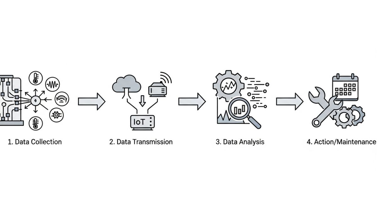
What is Condition-Based Maintenance and How Does It Work?
In my 20-plus years of managing piping systems, high-pressure pumps, and heavy rotating machinery, I have seen millions of dollars literally vanish due to unexpected equipment failures. Traditional calendar-based maintenance schedules often lead to over-maintaining healthy assets or, worse, missing a catastrophic failure by just a few days. That is where condition-based maintenance changes the game. By listening to the machine itself, we let real-time physical parameters dictate our maintenance windows.
When we transition a plant from reactive run-to-failure modes to a structured condition-based maintenance framework, we are not guessing. We rely on physical indicators like vibration velocity, oil particulate counts, and thermal signatures. This approach ensures that we only open up a pump or replace a piping spool when the data proves it is necessary, preserving the mechanical integrity of the system and avoiding infant mortality failures caused by unnecessary maintenance interventions.
Key Takeaways for Plant Engineers
- Real-time data acquisition eliminates the guesswork of calendar-based PM schedules.
- Compliance with standards like ISO 17359 provides a structured framework for asset health monitoring.
- Early detection of bearing wear, cavitation, and structural fatigue saves up to 40% in maintenance costs.
Complete Course on
Piping Engineering
Check Now
Key Features
- 125+ Hours Content
- 500+ Recorded Lectures
- 20+ Years Exp.
- Lifetime Access
Coverage
- Codes & Standards
- Layouts & Design
- Material Eng.
- Stress Analysis
Implementing Condition-Based Maintenance in Industrial Plants
To successfully deploy condition-based maintenance, we must first understand the physical degradation mechanisms of our assets. For rotating equipment like centrifugal pumps, the primary failure modes occur in the bearings and shaft seals. By mounting piezoelectric accelerometers directly to the bearing housing, we capture high-frequency vibration signals that indicate early-stage pitting, spalling, or misalignment.
The Physics of Vibration Monitoring
In my field work, we calculate the Root Mean Square (RMS) vibration velocity to assess overall machine health. The RMS velocity represents the energy content of the vibration signal and is calculated using the following mathematical relationship:
Where:
– v_rms is the root-mean-square vibration velocity (mm/s or in/s).
– T is the sampling period.
– v(t) is the time-dependent vibration velocity signal.
When the v_rms value exceeds the thresholds defined in ISO 10816-3, it indicates a transition from Zone A (new machine condition) to Zone C (unsatisfactory) or Zone D (unacceptable, risk of immediate damage).
Calculating Bearing Life Reduction Under Dynamic Load
Unbalance and misalignment introduce dynamic forces that drastically reduce bearing life. The L10 nominal rating life of a rolling element bearing is calculated using the basic rating life equation:
Where:
– L10 is the basic rating life in operating hours.
– C is the basic dynamic load rating (Newtons), provided by the manufacturer.
– P is the equivalent dynamic bearing load (Newtons).
– p is the life exponent (3 for ball bearings, 10/3 for roller bearings).
– n is the rotational speed in RPM.
If a pump experiences severe misalignment, the equivalent dynamic load (P) can double. Because of the cubic exponent (p = 3) for ball bearings, doubling the load reduces the bearing life to one-eighth (12.5%) of its original design life. This mathematical reality highlights why real-time detection via condition-based maintenance is so critical.
Acoustic Emission and Oil Analysis Integration
For low-speed machinery (under 100 RPM), standard vibration accelerometers often fail to capture the low-energy signals of early wear. In these scenarios, we utilize acoustic emission (AE) sensors operating in the 100 kHz to 1 MHz range. These sensors detect the elastic waves generated by micro-cracking and friction.
Simultaneously, online oil tribology sensors track metallic wear debris, moisture contamination, and oil viscosity. This multi-parametric approach ensures that we catch failures in complex piping and pumping systems long before they lead to catastrophic loss of containment.
The table below outlines the vibration velocity limits (RMS in mm/s) for different machine groups. This standard serves as the baseline for configuring alarm thresholds in condition-based maintenance software.
| Machine Group | Zone A (Good) | Zone B (Satisfactory) | Zone C (Unsatisfactory) | Zone D (Unacceptable) |
|---|---|---|---|---|
| Group 1: Large Pumps & Motors (>300 kW) | < 2.3 mm/s | 2.3 to 4.5 mm/s | 4.5 to 7.1 mm/s | > 7.1 mm/s |
| Group 2: Medium Pumps & Motors (15 to 300 kW) | < 1.4 mm/s | 1.4 to 2.8 mm/s | 2.8 to 4.5 mm/s | > 4.5 mm/s |
| Group 3: Pumps with Radial/Axial Flow Impellers | < 1.8 mm/s | 1.8 to 3.5 mm/s | 3.5 to 5.6 mm/s | > 5.6 mm/s |
This matrix maps specific physical parameters to their corresponding sensor technologies, diagnostic standards, and typical industrial applications.
| Physical Parameter | Sensor Technology | Standard Reference | Target Failure Mode |
|---|---|---|---|
| Vibration Velocity & Acceleration | Piezoelectric Accelerometers | ISO 10816-3 | Unbalance, misalignment, bearing wear, structural looseness |
| Acoustic Emission (AE) | High-Frequency AE Transducers | ISO 22096 | Micro-cracking, valve leakage, cavitation, low-speed bearing wear |
| Thermal Signature | Infrared Cameras & RTDs | ISO 18434-1 | Electrical imbalances, insulation degradation, friction heating |
| Oil Contamination | Laser Particle Counters | ISO 4406 | Abrasive wear, water ingress, additive depletion |
Deploying Condition-Based Maintenance Field Verification Steps
Before you trust your plant’s safety to an automated monitoring system, you must verify that the physical installation is flawless. A poorly mounted sensor will feed garbage data into your predictive models, leading to missed failures or costly false alarms. Use this checklist during your next field commissioning cycle.
Sensor Installation & Calibration Checklist
-
Surface Preparation: Ensure the mounting surface is machined flat to a surface roughness of less than 3.2 micrometers (125 micro-inches) to prevent high-frequency signal attenuation.
-
Mounting Torque Verification: Verify that stud-mounted accelerometers are torqued to the exact manufacturer specification (typically 2.3 to 3.4 Nm) using a calibrated torque wrench.
-
Coaxial Cable Protection: Route all sensor cables through flexible, liquid-tight conduit to protect against mechanical damage, chemical exposure, and electromagnetic interference (EMI) in compliance with NFPA 70 (NEC).
-
Data Acquisition Calibration: Perform a loop check from the sensor head to the PLC/SCADA input card using a handheld shaker table to verify amplitude and frequency accuracy.
-
Baseline Signature Capture: Record the initial “healthy” baseline spectrum under normal operating loads and speeds to establish the reference profile for future anomaly detection.
Field Case Study: Real-World Application
The Problem: Cavitation-Induced Piping Fatigue
At a major petrochemical facility, a high-pressure boiler feed pump bypass line was experiencing severe, intermittent vibration. The plant was operating on a standard 12-month preventive maintenance cycle. Within 4 months of a major overhaul, the piping system suffered a fatigue crack at a socket-welded drain connection, resulting in a high-pressure steam leak and an emergency plant shutdown. The cost of the unscheduled shutdown exceeded 280,000 in lost production.
The Solution: Dynamic Strain and Acoustic Monitoring
Instead of simply repairing the weld and waiting for the next failure, we installed a real-time condition-based maintenance system. We mounted dynamic strain gauges near the high-stress weld joints and high-frequency acoustic emission sensors on the control valve body.
Within three weeks of installation, the acoustic emission sensors detected high-frequency stress waves characteristic of micro-cavitation inside the valve. The dynamic strain gauges recorded peak-to-peak stress amplitudes approaching the fatigue limit of the carbon steel piping (defined by ASME B31.3).
Direct Engineering Recommendation
The real-time data allowed us to identify that the cavitation occurred only when the bypass valve operated at less than 15% open. We modified the control system logic to prevent the valve from dwelling in this critical zone. By implementing this condition-based maintenance strategy, we eliminated the piping fatigue mechanism entirely, saving the plant an estimated 150,000 annually in repair costs and preventing future catastrophic failures.
Frequently Asked Engineering Questions
What is the difference between predictive maintenance and condition-based maintenance?
Which standards govern the implementation of CBM systems?
How do you prevent false alarms in a CBM system?
Can CBM be applied to static equipment like piping and pressure vessels?
What are the limitations of condition-based maintenance?
How does CBM improve safety in hazardous environments?
===

📚 Recommended Resources: condition-based maintenance

Related posts:
![Industrial worker welding a large structural steel I-beam in a fabrication facility.]()
What is Structural Steel Fabrication and How Does It Work?
![A heavy-duty stainless steel turnbuckle tensioning a structural cable.]()
What is a Turnbuckle and How to Install It?
![Stack of newly manufactured galvanized steel pipes in an industrial warehouse]()
Understanding the Galvanized Pipe Meaning in Modern Piping Systems
![Industrial Alloy 625 piping components in a manufacturing plant]()
What is Alloy 625? Properties, Grades, and Applications of Alloy 625
![Close-up of a fractured steel shaft showing metal fatigue beach marks and failure zones.]()
What is Metal Fatigue and How Do Engineers Prevent It?
![Comparison of high viscosity honey and low viscosity water pouring to demonstrate fluid resistance]()
Understanding Newton's Law of Viscosity and Key Fluid Flow Factors