Flow through Pipes: Engineering Guide to Fluid Properties & System Effects

Imagine a massive offshore platform where a sudden 10% increase in crude viscosity stalls the entire production line because the original pump curves didn’t account for temperature-dependent Flow through Pipes. It’s not just about moving liquid from point A to B; it’s about managing the invisible forces of friction, turbulence, and pressure that can either optimize a plant or lead to catastrophic cavitation. In this guide, we bridge the gap between textbook fluid mechanics and 2026 field reality.
Key Takeaways
- Identify how Reynolds Number dictates the transition from laminar to turbulent regimes.
- Quantify the impact of pipe roughness and fluid viscosity on total system head loss.
- Apply 2026 calculation methodologies for both series and parallel piping networks.
What is Flow through Pipes?
Flow through Pipes is a branch of fluid mechanics concerned with the movement of liquids and gases through enclosed conduits. It is governed by the principles of conservation of mass, energy, and momentum, where flow behavior is primarily determined by fluid velocity, pipe diameter, and viscosity (Reynolds Number).
Founder’s Insight
“In my 20 years of piping design, I’ve seen more errors in Flow through Pipes calculations due to ignoring ‘Minor Losses’ in valves than in the actual pipe friction. Never underestimate the K-factor of a partially closed gate valve.”
— Atul Singla
Table of Contents
Complete Course on
Piping Engineering
Check Now
Key Features
- 125+ Hours Content
- 500+ Recorded Lectures
- 20+ Years Exp.
- Lifetime Access
Coverage
- Codes & Standards
- Layouts & Design
- Material Eng.
- Stress Analysis
Knowledge Check: Flow through Pipes
Question 1 of 51. Which dimensionless number is primarily used to determine if the Flow through Pipes is laminar or turbulent?
Fundamental Mechanics of Flow through Pipes
Understanding the physics of Flow through Pipes requires a deep dive into fluid dynamics and thermodynamics. At its core, the movement of any substance—whether liquid or gas—through a conduit is driven by a pressure gradient. In industrial engineering, we analyze this behavior using the Continuity Equation and Bernoulli’s Principle. For an incompressible fluid, the mass flow rate remains constant throughout the system, meaning that any reduction in pipe cross-sectional area must result in a proportional increase in fluid velocity. This relationship is critical when sizing nozzles or venturing into venturi meter designs within a complex piping network.
Defining the Fluid: Properties Shaping Flow through Pipes
The efficiency of Flow through Pipes is dictated by the inherent physical properties of the medium. Viscosity stands as the most influential factor; it represents the internal resistance of the fluid to shear or flow. High-viscosity fluids, like heavy crude oil, require significantly more pumping power to overcome the "internal friction" compared to low-viscosity fluids like water. Furthermore, Density and Specific Gravity play vital roles in determining the Reynolds Number and the resulting pressure drop. According to the ASME Standards, understanding the temperature-dependence of these properties is non-negotiable for safe system operation, as fluid density and viscosity shift dramatically under varying thermal conditions.
Internal Dynamics: Fluid Flow inside Pipeline Systems
When we examine Flow through Pipes at a granular level, we observe the "No-Slip Condition." This principle dictates that the fluid layer in direct contact with the pipe wall has zero velocity relative to the pipe. This creates a velocity profile across the pipe diameter. In a fully developed flow, this profile becomes predictable, allowing engineers to calculate the average velocity used in discharge formulas. The boundary layer growth, which starts at the pipe entrance, eventually merges at the centerline to establish what is known as "fully developed flow." For modern piping designers, identifying the entrance length is essential to ensure that flow meters are placed in regions where the velocity profile is stable and accurate readings are possible.
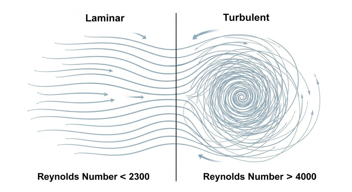
Laminar vs Turbulent: How does Fluid Flow in Pipes?
The regime of Flow through Pipes is categorized into two distinct states: Laminar and Turbulent. Laminar flow occurs at low velocities where fluid particles move in smooth, parallel layers (laminae) with no macroscopic mixing. This usually occurs when the Reynolds Number (Re) is below 2,100. Conversely, Turbulent flow occurs when Re exceeds 4,000, characterized by chaotic eddy currents and rapid mixing. The transition zone (2,100 < Re < 4,000) is a critical area for engineers to monitor, as flow behavior here can be unpredictable. Most industrial applications favor turbulent flow because it enhances heat transfer and mixing, despite the higher frictional losses associated with chaotic particle motion.
Engineering Math: Essential Pipe Flow Calculations
Calculating the discharge and velocity of Flow through Pipes is the backbone of hydraulic design. The primary formula utilized is Q = A × V, where Q is the volumetric flow rate, A is the cross-sectional area, and V is the mean velocity. To calculate the pressure drop required to maintain this flow, engineers frequently turn to the Hazen-Williams or Darcy-Weisbach equations. In 2026, computational fluid dynamics (CFD) has simplified these iterations, but the manual verification of Reynolds Numbers remains a foundational skill for any professional listed on the API Standards rosters to ensure compliance with safety and efficiency benchmarks.
Analyzing Friction and Major Losses in Flow through Pipes
In any industrial Flow through Pipes, energy is lost primarily due to friction between the fluid and the pipe wall. This is termed "Major Loss." The Darcy-Weisbach equation remains the gold standard for calculating this pressure drop. It factors in the Darcy friction factor (f), which for turbulent flow, is a function of the Relative Roughness of the pipe material. Engineering standards like ASME B31.3 Process Piping mandate strict adherence to these calculations to ensure structural integrity under pressure. Minor losses, caused by valves, bends, and tees, are equally critical and are typically quantified using the Resistance Coefficient (K-factor) or the equivalent length method.
Gas Flow through Piping Systems: Compressibility Factors
Unlike liquids, Flow through Pipes involving gases must account for Compressibility. As gas moves through a pipeline, pressure drops and velocity increases, leading to changes in density. For high-pressure natural gas transmission, engineers must reference API 570 Inspection Standards to monitor for erosion-corrosion caused by high-velocity gas streams. In 2026, the use of the Weymouth and Panhandle equations is still standard practice for long-distance gas pipelines, where isothermal or adiabatic flow conditions are assumed based on the insulation and burial depth of the system.
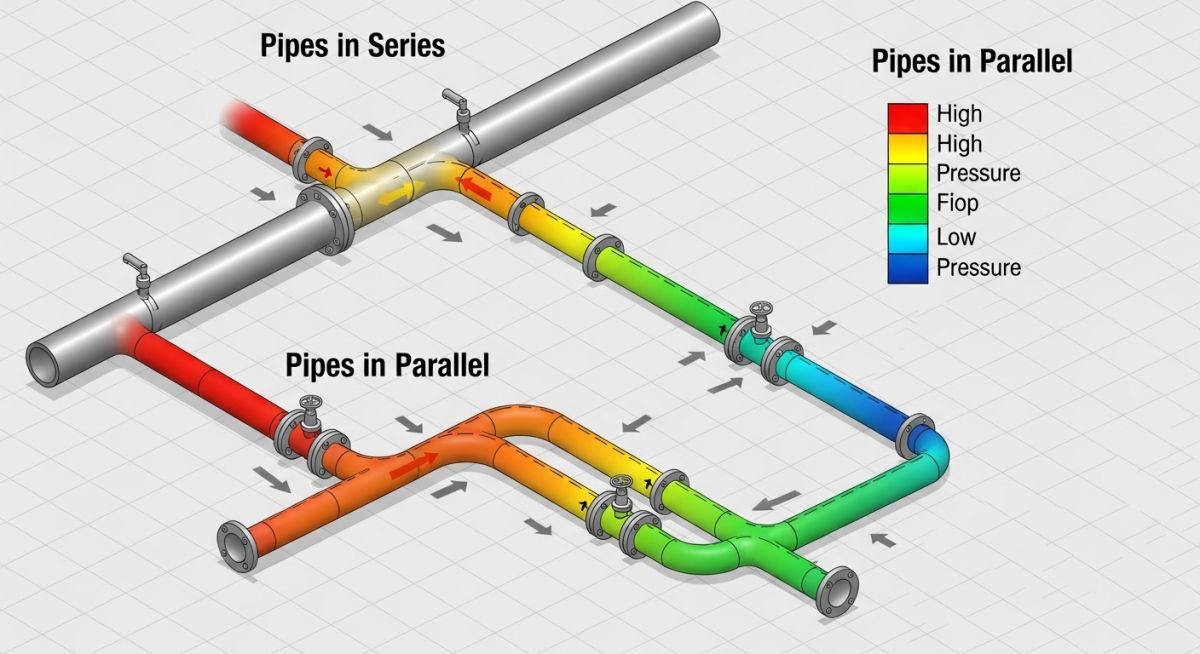
Network Analysis: Flow through Pipes in Series and Parallel
Complex industrial plants rarely rely on a single line; they utilize networks. When analyzing Flow through Pipes in series, the flow rate (Q) remains constant across all sections, while the total head loss is the sum of losses in each pipe. Conversely, for pipes in parallel, the pressure drop across each branch is identical, but the total flow rate is divided among the branches based on their individual resistances. This is analogous to Kirchhoff’s laws in electrical circuits and is essential for designing redundant cooling systems or manifold distributions.
| Parameter | Pipes in Series | Pipes in Parallel |
|---|---|---|
| Flow Rate (Q) | Qtotal = Q1 = Q2 = Qn | Qtotal = Q1 + Q2 + Qn |
| Head Loss (hL) | hL-total = hL1 + hL2 + hL3 | hL-total = hL1 = hL2 = hL3 |
| Primary Design Goal | Transport across distances | System redundancy & pressure stability |
| System Resistance | Cumulative increase | Reduced overall resistance |
Expert Course: Mastering Flow through Pipes, Valves, and Pumps
For engineers looking to dominate the 2026 job market, theoretical knowledge is only the starting point. Our comprehensive online course on Flow through Pipes provides hands-on simulation training for real-world scenarios. We cover advanced topics like water hammer analysis, non-Newtonian fluid behavior, and the integration of ISO 15649 standards for piping design. Whether you are troubleshooting an existing line or designing a new process facility, mastering these fluid properties is your key to operational excellence.
Reynolds Number Calculator
Determine if your Flow through Pipes is Laminar, Transitional, or Turbulent.
Optimization of High-Viscosity Crude Transfer: A 2026 Analysis
The Problem
An onshore terminal experienced a 40% reduction in discharge flow rate during winter months. Initial assessments blamed pump wear, but the issue was rooted in the Flow through Pipes dynamics of the heavy crude.
The Investigation
Analysis revealed that ambient temperature drops increased fluid viscosity from 200 cSt to 850 cSt, shifting the Reynolds Number from the turbulent regime into the transitional zone.
The Solution
Instead of replacing pumps, engineers installed high-efficiency heat tracing and transitioned the piping manifold from a series to a parallel configuration to reduce total system resistance.
Engineering Results
By manipulating the variables of Flow through Pipes, the facility achieved a stable flow rate without increasing energy consumption. The parallel manifold reduced the head loss by approximately 65%, allowing the existing pumps to operate at their Best Efficiency Point (BEP).
Lesson Learned: Temperature control is the most cost-effective way to manage frictional losses in high-viscosity piping systems.
EPCLand YouTube Channel
2,500+ Videos • Daily Updates
Expert Insights: Lessons from 20 years in the field
Don't trust nominal diameters: When calculating Flow through Pipes for high-pressure systems, always use the internal diameter (ID) based on the specific pipe schedule. A Schedule 160 pipe has significantly less flow area than a Schedule 40 of the same nominal size, which drastically increases velocity and pressure drop.
The Roughness Reality: The Darcy Friction Factor is not static. In 2026, we increasingly see "aged" pipe friction values being ignored in the design phase. Always include a safety margin for internal scaling and corrosion, as the relative roughness of steel pipe can double after just 5 years of service.
Check for Cavitation: If your Flow through Pipes involves a high-point in the layout, ensure the local pressure doesn't drop below the fluid's vapor pressure. I have seen multi-million dollar pump systems destroyed because an engineer ignored the elevation head loss at the system apex.
Frequently Asked Questions: Flow through Pipes
What causes the most pressure drop in Flow through Pipes?
How do you calculate the flow rate through a pipe?
Why is the Reynolds Number important for piping design?
In 2026, should I use the Hazen-Williams or Darcy-Weisbach equation?
How does internal pipe corrosion affect Flow through Pipes over time?
What is the "No-Slip" condition in practical piping engineering?

Related posts:
![High-grade industrial Wing Nut Types and Applications for mechanical assemblies.]()
Wing Nut Types and Applications: The 2026 Engineering Guide
![Industrial Monorail Crane Systems installed in a modern manufacturing plant 2026.]()
Monorail Crane Systems: Design, Types & 2026 Standards Guide
![Lead engineer performing a Factory Acceptance Test FAT on an industrial skid system 2026]()
Factory Acceptance Test FAT: The 2026 Engineering Guide to Zero-Defect Delivery
![Professional engineering workspace showing a Basis of Design document layout for a 2026 project.]()
Basis of Design: How to Write a BOD for Engineering Projects in 2026
![Industrial Flare Knockout Drum Sizing and installation in a refinery relief system.]()
Flare Knockout Drum Sizing: Design & API 521 Standards (2026 Guide)
![Advanced Reboiler Control Systems in a modern petrochemical refinery 2026.]()
Reboiler Control Systems: Engineering Guide to Precision Control 2026